I just started a new role as a Staff Product Manager. Day one was approaching fast, and I had a blank MacBook Pro sitting on my desk. A 14-inch M4 Pro with 24GB of RAM and a 512GB SSD.
The question wasn’t what to install. It was how to set up a machine that lets a PM move at the speed of thought: writing PRDs to spinning up prototypes to jumping on a customer call, all without friction.
This is the guide I wish I’d had.
0
Tools Installed
0
Hour to Set Up
0
Excuses Left
The PM’s Dilemma
There’s a tension at the heart of every PM’s toolkit. You’re not an engineer, but you need to speak their language. You’re not a designer, but you need to give precise feedback. You’re not in sales, but you need to demo the product on the fly.
My philosophy is simple:
Be technical enough to prototype, clear enough to document, and fast enough to never block your team.
That means optimizing for speed, clarity, and collaboration, not engineering perfection. Every tool below earns its place by making me faster at one of three jobs:
- Writing. PRDs, specs, customer insights
- Building. Prototypes, MVPs, proof-of-concepts
- Communicating. Demos, presentations, async updates
The Machine
Hardware
MacBook Pro 14″ / M4 Pro
macOS Sequoia 15.4.1
Why does a PM need an M4 Pro? Because on any given Tuesday I’m running Docker containers, Figma with a 200-screen file, 40 browser tabs of customer research, a Zoom call, and a local AI model. All at once, without the fans spinning up.
First Things First: System Preferences
Before installing a single app, I spend 20 minutes dialing in macOS itself. These tweaks are small individually, but compound into a noticeably smoother experience.
Look & Feel
Dark mode, always. Auto-hide the Dock. Remove every app I won’t use daily. Show battery percentage. Turn on Night Shift for late writing sessions.
Notifications: The Great Silencing
I keep exactly three apps allowed to interrupt me: Calendar (meetings), Slack (team comms), and Linear (project updates). Everything else gets turned off. Context switching is the PM’s worst enemy.
Trackpad
System Settings → Trackpad. Max tracking speed. Enable Tap to Click. These two changes alone make the MacBook feel twice as responsive.
Mouse
If you’re using an Apple Mouse with your Apple Studio Display (or standalone), head to System Settings → Mouse. Enable Secondary Click and set it to Click Right Side. Right-click is essential for context menus everywhere, from Figma to the terminal.
Keyboard Shortcuts
System Settings → Keyboard → Keyboard Shortcuts → Spotlight: disable Spotlight’s Cmd+Space shortcut. We’re replacing it with something much better.
Finder
Open Finder, then go to Finder → Settings (Cmd+,). A few tweaks that save daily friction:
- General tab. Set “New Finder windows show” to Downloads
- Advanced tab. Check “Show all filename extensions” and set “Remove items from the Bin after 30 days”
- Desktop. Keep it completely empty. No files, no folders. If something’s on the desktop, it doesn’t have a home yet.
Security
Non-negotiable: FileVault ON (full disk encryption), Touch ID for everything. If you’re handling customer data, competitive intel, or roadmap docs (and you are), encryption isn’t optional.
Get a password manager. 1Password is my pick. It handles passwords, SSH keys, API tokens, and secure notes in one place. Bitwarden is a solid free alternative. Either way, stop reusing passwords and storing secrets in plain text files.
Terminal Tweaks
A handful of defaults write commands that macOS should ship with out of the box:
# Screenshots as JPG (smaller, good enough)
defaults write com.apple.screencapture type jpg

# Show hidden files, path bar, status bar in Finder
defaults write com.apple.finder AppleShowAllFiles YES
defaults write com.apple.finder ShowPathbar -bool true
defaults write com.apple.finder ShowStatusBar -bool true

# Unhide the Library folder
chflags nohidden ~/Library

killall Finder
The Foundation: Homebrew
Everything starts here. One command to install the macOS package manager that makes everything else possible:
/bin/bash -c "$(curl -fsSL \
  https://raw.githubusercontent.com/Homebrew/install/HEAD/install.sh)"
From this point on, installing software is just brew install or brew install --cask. No more dragging .dmg files around.
The App Stack
Here’s where things get opinionated. I split my apps into two categories: GUI apps I interact with visually, and terminal tools that power my command-line workflows.
GUI Apps: One Command
As of this writing, these are my current preferences. They change over time, so check the last updated date at the top.
brew install --cask \
  raycast google-chrome arc firefox \
  ghostty visual-studio-code cursor \
  figma notion linear-linear \
  slack discord zoom loom \
  cleanshot rectangle obsidian \
  tableplus postman docker \
  1password vlc maccy imageoptim
That’s 24 apps installed in under a minute. Let me walk through the ones that matter most.
Terminal Tools
brew install \
  git gh wget nvm pnpm yarn \
  jq tree htop tlrc bat \
  fzf ripgrep eza claude-code
These are the quiet workhorses. bat is a better cat. eza is a better ls. fzf is fuzzy finding for everything. tlrc gives you practical examples instead of man pages. ripgrep searches code faster than you can think of what to search for.
Deep Dives: The Tools That Changed My Workflow
Raycast: The Command Center
This is the single most impactful app on this list. Raycast replaces Spotlight with something that actually understands how you work.
Cmd+Space opens it. From there I can:
- Search files, apps, and bookmarks instantly
- View my calendar without opening Calendar
- Search Linear issues or Notion docs
- Manage windows without reaching for a mouse
- Access clipboard history (every URL, quote, and snippet I’ve copied today)
The Browser Trinity
I use three browsers, each with a distinct job:
Chrome is my primary. The dev tools are unmatched. Extensions: 1Password, uBlock Origin, React DevTools, JSON Viewer, Loom, Notion Web Clipper, Grammarly, and a design QA trio: ColorZilla, WhatFont, Page Ruler.
Arc is for research. Its Spaces feature lets me keep separate contexts (competitive research, customer interviews, documentation) without drowning in tabs.
Firefox Developer Edition is for cross-browser testing. Because “it works on Chrome” isn’t a shipping standard.
The Terminal: Ghostty + Oh My Zsh + Starship
The default Terminal app is fine. Ghostty is better. It’s fast, memory-efficient, and GPU-accelerated. Split panes, native macOS feel, and none of the bloat.
Layer on Oh My Zsh for plugin management and Starship for a beautiful, informative prompt:
# Oh My Zsh
sh -c "$(curl -fsSL \
  https://raw.githubusercontent.com/ohmyzsh/ohmyzsh/master/tools/install.sh)"

# Starship prompt
brew install starship
echo 'eval "$(starship init zsh)"' >> ~/.zshrc

# Hack Nerd Font (for icons in the prompt)
brew install --cask font-hack-nerd-font
Essential Plugins
Three plugins that make the terminal feel like it can read your mind:
- zsh-autosuggestions suggests commands as you type based on history
- zsh-syntax-highlighting colors valid commands green, invalid ones red
- zsh-completions smarter tab completion
These are custom plugins, so you need to clone them first:
git clone https://github.com/zsh-users/zsh-autosuggestions \
  ${ZSH_CUSTOM:-~/.oh-my-zsh/custom}/plugins/zsh-autosuggestions

git clone https://github.com/zsh-users/zsh-syntax-highlighting \
  ${ZSH_CUSTOM:-~/.oh-my-zsh/custom}/plugins/zsh-syntax-highlighting

git clone https://github.com/zsh-users/zsh-completions \
  ${ZSH_CUSTOM:-~/.oh-my-zsh/custom}/plugins/zsh-completions
Then add them to your plugin list in ~/.zshrc:
plugins=(
  git
  zsh-completions
  zsh-autosuggestions
  zsh-syntax-highlighting
  docker
  npm
)
My Aliases
These save me hundreds of keystrokes a day:
# Git (the ones I actually use)
alias gs="git status"
alias ga="git add ."
alias gc="git commit -m"
alias gp="git push"
alias gl="git lg"

# Navigation
alias projects="cd ~/Projects"
alias work="cd ~/Projects/work"

# Utilities
alias week="date +%V"
alias serve="python3 -m http.server 8000"
VS Code: The Writing & Coding Workhorse
Although a traditional IDE is needed less and less with AI-powered tools like Cursor and Claude Code handling most of the heavy lifting, I’m still using VS Code to manually review and update code. Honestly, I expect this section to be removed in the next six months.
For now, VS Code is where I spend a good chunk of my day. Not just for code. I use it for Markdown, JSON, YAML, meeting notes, and PRDs.
Extensions That Matter for PMs
Writing
- Markdown All in One
- Code Spell Checker
- Prettier
- Better Comments
Product Work
- GitLens
- TODO Highlight
- Project Manager
- Bookmarks
Development
- GitHub Copilot
- ESLint
- Error Lens
- Auto Close/Rename Tag
Productivity
- Auto Hide Sidebar
- FontSize Shortcuts
- Formatting Toggle
- Path Intellisense
Key Settings
A few settings that make VS Code feel like a focused writing environment, not an IDE:
{
  "editor.fontSize": 14,
  "editor.fontFamily": "Hack Nerd Font Mono",
  "editor.minimap.enabled": false,
  "editor.padding.top": 36,
  "workbench.colorTheme": "GitHub Dark Default",
  "workbench.sideBar.location": "right",
  "workbench.activityBar.location": "hidden",
  "files.autoSave": "afterDelay",
  "files.autoSaveDelay": 1000,
  "[markdown]": {
    "editor.formatOnSave": false,
    "editor.wordWrap": "on"
  }
}
Sidebar on the right. Activity bar hidden. Minimap off. Auto-save on. It’s a writing tool that happens to also run code.
The AI Layer: Cursor + Claude Code
This is the 2025 part. Two tools that didn’t exist in my setup a year ago, and now I can’t imagine working without them.
Cursor: AI-First Editor
For rapid prototyping and MVP development. When I need to go from “idea on a whiteboard” to “working prototype” in an afternoon, Cursor is where it happens.
- Generate boilerplate for proof-of-concepts
- Explain unfamiliar codebases I’m reviewing
- Draft API schemas and data models
- Turn a sketch into a functional component
Claude Code: The Terminal Agent
This is the tool that changed how I work. Claude Code lives in my terminal and handles complex, multi-step coding tasks autonomously. Currently running with Opus 4.6, it’s the best I’ve found for handling PRDs and building quick MVPs.
npm install -g @anthropic-ai/claude-codeWhat I actually use it for:
# Generate a PRD from rough notes
claude "Create a comprehensive PRD for 'user-authentication'
  with problem statement, user stories, success metrics,
  and technical considerations"

# Analyze customer feedback
claude "Analyze this feedback file. Extract themes,
  pain points, feature requests, and sentiment"
  customer-feedback.txt

# Scaffold a prototype
claude "Build a landing page with hero, features,
and CTA using Tailwind CSS"The Supporting Cast
These tools don’t get the headlines, but they keep everything running smoothly.
Notion
Documentation hub. PRD templates, meeting notes, customer interview databases, competitive analysis. The single source of truth for everything written.
Obsidian
Personal knowledge management. Local-first, Markdown-based. Where I build my “second brain”: daily notes, product insights, reading notes, patterns I notice across customer calls.
Figma
Design collaboration. Review designs, create quick wireframes, annotate with feedback, prototype simple flows. Learn the shortcuts: C for comments, V for move.
Linear
Issue tracking that doesn’t feel like punishment. Keyboard-driven, fast, beautiful. C to create, / to search. Custom views per project.
CleanShot X
Screenshots and screen recording that’s better than macOS built-in in every way. Annotate instantly, record GIFs for bug reports, scrolling capture for long pages.
Loom
Async video for remote PMs. Share product demos, give design feedback, explain complex concepts, all without scheduling a meeting.
Rectangle + Maccy
Window management via keyboard (Ctrl+Opt+arrows) and clipboard history (Cmd+Shift+V). Small tools, massive time savings.
Docker Desktop
Containers for local development. Run databases, APIs, and full-stack apps without polluting your system. It’s the quickest way to get a reproducible dev environment. Worth noting: if your team runs Kubernetes in production, Rancher Desktop (free, ships with k3s) might be a better fit. Podman is another solid alternative if you want something lighter and daemonless.
TablePlus + Postman
Database GUI and API testing. For when you need to verify metrics, understand data models, or test endpoints yourself. Read-only production access is your friend.
Developer Essentials: Git, SSH & Node
Even as a PM, these are non-negotiable. You need to clone repos, review PRs, and run prototypes locally.
Git Configuration
git config --global user.name "Murat Karslioglu"
git config --global user.email "your-email@company.com"
git config --global init.defaultBranch main

# A beautiful git log
git config --global alias.lg "log --color --graph \
  --pretty=format:'%Cred%h%Creset -%C(yellow)%d%Creset \
  %s %Cgreen(%cr) %C(bold blue)<%an>%Creset' \
  --abbrev-commit"
SSH for GitHub
ssh-keygen -t ed25519 -C "github"
ssh-add --apple-use-keychain ~/.ssh/github

# Add to GitHub with the CLI
gh auth login
gh ssh-key add ~/.ssh/github.pub -t github
Node.js for Prototyping
# Install via NVM (version manager)
nvm install --lts
node -v && npm -v

# Global tools for quick prototyping
npm install -g serve http-server \
json-server netlify-cli vercelThe Workflows That Tie It All Together
Tools are nothing without workflows. Here are the three I run on repeat.
The Morning Routine
pmsetupin the terminal: starts Docker, opens Notion, Linear, Slack- Cmd+Space → “cal” to review today’s meetings in Raycast
- Check Linear for overnight updates
- Open Daily Note in Obsidian
- Start working on the highest-impact item
The Documentation Flow
Customer call → Loom recording → transcribe with Otter.ai → extract insights into Notion → synthesize patterns in Obsidian → update the PRD
Every insight has a clear path from conversation to product decision.
The Prototype Flow
Sketch in FigJam → mockup in Figma → build in Cursor or with Claude Code → deploy to Vercel → share a Loom walkthrough
From idea to deployed prototype, tested with real users, in a single day.
The Folder Structure
Simple, predictable, and hard to mess up:
~/Projects/
├── work/            # Company projects
│   ├── docs/        # Internal documentation
│   ├── prototypes/  # Quick MVPs
│   └── research/    # Customer interviews, analysis
├── blog/            # Personal blog
├── learning/        # Courses, tutorials
└── personal/        # Side projects
Everything has a home. Nothing lives on the Desktop.
Keeping It Running: Maintenance
A setup is only as good as its maintenance. I follow a simple cadence:
Weekly: brew update && brew upgrade, clear Downloads, archive old Notion pages, push Obsidian vault to GitHub.
Monthly: Update VS Code extensions, remove unused apps, clear browser caches, npm update -g.
Quarterly: macOS system update, audit installed apps, review security settings, clean up SSH keys.
Backup strategy: Code lives on GitHub. Documents in Notion + Google Drive. Personal notes in Obsidian (synced to GitHub). Passwords in 1Password. Config files in a dotfiles repo. Time Machine to an external SSD for everything else.
Your First Week Checklist
If you’re starting a new PM role, here’s what to get done in week one:
- All system access: Slack, Linear/Jira, Figma, Notion, repos
- SSH keys configured, VPN set up
- Dev environment tested. Can you clone and run the product locally?
- First PRD template created in Notion
- Met with your engineering lead
- Reviewed the product roadmap
- Set up your customer feedback pipeline
The Bottom Line
This setup takes about an hour from a blank MacBook to a fully operational PM workstation. It balances three things:
Technical
Build MVPs, understand the stack, speak the team’s language
Clear
Write PRDs, present effectively, document thoroughly
Fast
Minimal friction, zero context switching, great tools
Tools don’t make you a great PM. Solving customer problems does. But great tools let you move faster and think clearer.
Now close this tab and go set up your machine.
The Beginning
Every personal site starts with a question: what do I actually want this to be?
I didn’t want a bloated portfolio template. I wanted something fast, clean, and focused on writing. Something that felt like opening a well-designed book.
Choosing the Stack
After evaluating several options, the choice was clear:
- Astro for its content-first approach and zero JS by default
- Tailwind CSS for rapid, consistent styling
- MDX for rich, interactive blog posts like this one
- GitHub Pages for simple, free hosting
0
Lighthouse Score
0 KB
KB of JavaScript
0
Pages Built
Design Principles
The design follows a few simple principles:
- Content first. Typography and readability above all else
- Minimal chrome. The interface should disappear
- Fast by default. No layout shifts, instant navigation
- Responsive everywhere. Works on any screen size
What’s Next
This site is a living project. I plan to keep iterating: adding new content, refining the design, and experimenting with new ways to tell stories on the web.
If you’re curious about the source code, it’s all on GitHub.
Thanks for scrolling along.
Welcome to my new website. I’ve been meaning to build this for a while, and here we are.
If the name rings a bell, you might remember me from containerized.me, where I used to write about the cloud-native world, Kubernetes, and container orchestration. I lost that domain when Google Domains went out of business. Honestly, I wasn’t updating it frequently anyway, so instead of chasing the old domain I’m starting fresh here. Hoping this time I’ll actually keep a regular cadence. We’ll see.
Why a Personal Site?
In the age of social media, having your own space on the internet feels more important than ever. It’s a place to think out loud, share what I’m learning, and connect with people who are curious about similar things.
What to Expect
I plan to write about a few topics that I spend most of my time thinking about:
- Product Management. Frameworks, processes, and lessons from building products
- Technology. Cloud-native infrastructure, Kubernetes, and developer tools
- Books. Reviews and takeaways from what I’m reading
- Building. The process of creating things, from software to teams
A Quick Example
Here’s a code snippet, because every developer blog needs one:
function buildSomethingGreat(idea: string): Product {
  const validated = validateWithUsers(idea);
  const prioritized = applyFramework(validated, "RICE");
  return ship(prioritized);
}
What’s Next
I’ll be publishing regularly, or at least that’s the plan. If any of this sounds interesting, stick around.
“The best time to plant a tree was twenty years ago. The second best time is now.”
Thanks for reading.

For 40 years, the CPU has been the I/O initiator for storage. It decides what gets read, when, and where it lands in memory. Every protocol in the stack assumes this: NVMe command queues, the Linux block layer, O_DIRECT, scatter-gather lists, interrupt-driven completions. All designed for a CPU host. AI inference is breaking that model. The GPU now knows what data it needs next (the next KV cache tensor, the next attention head), and routing that request through the CPU adds microseconds of latency that the GPU can’t afford. GPU-initiated I/O, direct NVMe reads over P2P DMA, is the architectural response. But the software stack wasn’t built for it, and the standards bodies haven’t caught up.
The CPU Was Always the I/O Initiator
Every storage architecture since the IBM PC/AT has followed the same flow: the CPU decides what data to fetch, builds a command descriptor, submits it to a device queue, and handles the completion interrupt. NVMe refined this model (65,535 queues, polling instead of interrupts, multi-core submission), but it didn’t change the fundamental assumption. The CPU is the host. The storage device is the target. Data flows from device to host memory, and if a GPU needs that data, the CPU copies it again.
This worked for 40 years because the CPU was the one doing the computation. It knew what data it needed because it was the one processing it. Even when GPUs became the dominant compute engines for training workloads, the data pipeline still made sense: the CPU prefetches training batches from storage, stages them in host DRAM, and the GPU pulls them over PCIe when ready. Training is sequential and predictable. You know which batch comes next because you designed the data loader.
Inference is different.
Why Inference Breaks the Model
Training reads data in large, predictable sequential sweeps. A DataLoader shuffles the dataset once per epoch, then streams batches in order. The CPU can prefetch effectively because the access pattern is known.
Inference generates its access pattern dynamically, one token at a time. Each forward pass through the model produces a new token, which changes what the next forward pass needs. And the dominant memory consumer in inference isn’t model weights (those are static, loaded once). It’s the KV cache.
The KV Cache Problem
Every transformer-based model maintains a key-value cache: the accumulated attention context from all previous tokens in the sequence. For each new token generated, the model reads the entire KV cache to compute attention, then appends the new token’s key-value pair. The cache grows linearly with sequence length.
The numbers are large and getting larger:
| Model | Context Length | KV Cache Size (FP16) | Notes |
|---|---|---|---|
| Llama 3.1 8B | 32K tokens | ~4 GB | Fits in single GPU HBM |
| Llama 3.1 8B | 128K tokens | ~16 GB | Still fits, barely |
| Llama 3.1 70B | 128K tokens | ~40 GB (with GQA) | Half of an H100’s HBM |
| Llama 3.1 70B | 128K tokens | ~320 GB (without GQA) | Exceeds any single GPU |
| Any 70B+ model | 1M tokens | ~150+ GB | Multi-GPU required |
GQA (Grouped Query Attention) and MLA (Multi-head Latent Attention) compress the KV cache by 4-8x, but the scaling problem remains. At 128K context, 4 concurrent requests on a Llama 70B model need roughly 160 GB of KV cache. That exceeds a single H200’s 141 GB of HBM. At 1M token context (which Claude, Gemini, and GPT-4 all support), the KV cache for a single session can exceed 15 GB with modern optimizations.
GPU HBM is precious. An H100 has 80 GB, an H200 has 141 GB, and a Blackwell B200 has 192 GB. Model weights for a 70B parameter model in FP16 consume ~140 GB alone. There is not enough HBM for both the model and all active KV caches. Something has to spill.
The Tiering Imperative
The industry’s answer is tiered KV cache storage. Hot cache stays in HBM. Warm cache spills to host DRAM. Cold cache goes to NVMe. The memory hierarchy that CXL is reshaping for storage metadata applies equally to inference state:
┌─────────────────────────────────────────────────────┐
│  GPU HBM          │  ~ns access   │  80-192 GB      │
│  (active KV)      │  TB/s BW      │  $$$$$           │
├─────────────────────────────────────────────────────┤
│  Host DRAM        │  ~μs access   │  512 GB - 2 TB  │
│  (warm KV)        │  ~26 GB/s     │  $$$             │
│                   │  (PCIe Gen4)  │                  │
├─────────────────────────────────────────────────────┤
│  Local NVMe       │  ~100 μs      │  4-60 TB        │
│  (cold KV)        │  7-14 GB/s    │  $$              │
├─────────────────────────────────────────────────────┤
│  Network Storage  │  ~ms access   │  Petabytes      │
│  (shared KV/ckpt) │  variable     │  $               │
└─────────────────────────────────────────────────────┘
The latency differences are brutal. vLLM’s KV offloading connector (v0.11.0+) measures 83.4 GB/s bidirectional transfer between GPU and CPU memory at 2 MB block sizes, yielding a 2-22x reduction in time-to-first-token for single requests. But that’s the best case, the DRAM tier. Moving KV cache from NVMe to GPU crosses both the PCIe bus and the NVMe latency floor, adding 100+ microseconds per I/O. FlexGen demonstrated only 1.9 tokens/s on NVMe for aggressive offloading, compared to KVSwap’s improved 6.9 tokens/s (2025) and vLLM’s 5x throughput gains through memory layout optimization (v0.12.0).
Every microsecond in this pipeline matters. And every microsecond the CPU spends mediating between the GPU and NVMe storage is a microsecond wasted.
The CPU Tax on GPU I/O
Here’s the path data takes today when a GPU needs a KV cache tensor from NVMe:
1. GPU signals CPU:     "I need KV block 47392"
2. CPU wakes up:        context switch, scheduler, driver entry
3. CPU builds NVMe cmd: allocate SQE, set LBA, set transfer size
4. CPU submits to SQ:   write SQE to submission queue, ring doorbell
5. NVMe processes:      read from flash, DMA to... where?
6. DMA to host DRAM:    NVMe writes to CPU-pinned bounce buffer
7. CPU copies to GPU:   cudaMemcpy() from host DRAM to GPU HBM
8. GPU resumes:         finally has the data, ~100-200 μs later
Steps 2, 3, 6, and 7 are pure overhead. The GPU knew what it needed. The NVMe drive could have DMA’d directly to GPU memory over PCIe. But the protocol stack requires the CPU to be the intermediary at every stage: building the command, managing the DMA target, handling the completion.
NVIDIA’s GPUDirect Storage (GDS) eliminates step 7. With GDS, NVMe data flows directly to GPU memory over PCIe, bypassing the host DRAM bounce buffer. GDS delivers up to 3.5x higher bandwidth and 3.5x lower latency compared to the CPU-mediated path. On a well-configured system, GDS sustains 84 GB/s across 10 NVMe drives per GPU, with peaks hitting 90 GB/s.
But GDS only removes the bounce buffer copy. The CPU still builds the NVMe commands. The CPU still submits them. The CPU still handles completions. The I/O initiation path is still CPU-bound.
For training workloads, where data access is predictable and can be prefetched in large batches, this is fine. The CPU pipelines NVMe reads far ahead of when the GPU needs the data. The GPU never stalls.
For inference, the GPU discovers what it needs during the forward pass. By the time it knows it needs KV block 47392, the decode step is already waiting. Routing that request through the CPU’s scheduler, driver stack, and NVMe submission path adds latency that directly impacts token generation speed. At 200M IOPS per GPU (the figure cited at LSFMM+BPF 2025 by storage engineers working on device-initiated I/O), the CPU simply cannot keep up. The NVMe driver handles 8-12M IOPS per core in IOMMU passthrough mode, dropping to roughly 2M IOPS with DMA mapping overhead. You’d need 25-100 CPU cores per GPU just for I/O submission. That’s absurd.
GPU-Initiated I/O: The Architectural Response
What if the GPU could submit NVMe commands directly, without waking the CPU at all?
This is GPU-initiated I/O. The concept: map the NVMe controller’s registers into GPU-accessible address space, place NVMe submission and completion queues in GPU memory, and let GPU threads build and submit I/O commands directly. The CPU handles setup (device discovery, queue creation, BAR mapping) but steps out of the data path entirely.
The path becomes:
1. GPU thread:          "I need KV block 47392"
2. GPU builds NVMe cmd: writes SQE directly to submission queue (in GPU memory)
3. GPU rings doorbell:  writes to NVMe BAR0 doorbell register (memory-mapped)
4. NVMe processes:      reads SQE from GPU memory via PCIe, reads flash
5. NVMe DMA to GPU:     writes data directly to GPU HBM via P2P PCIe
6. GPU polls CQ:        reads completion entry from CQ (in GPU memory)
7. GPU resumes:         has the data
No CPU involvement on the data path. No context switches. No bounce buffers. No cudaMemcpy. The entire I/O round-trip happens over the PCIe bus between two devices, with the GPU as the initiator.
BaM: The Proof It Works
The most rigorous demonstration of GPU-initiated I/O is BaM (Big accelerator Memory), published at ASPLOS 2023 by researchers from NVIDIA and the University of Illinois. BaM moves NVMe submission and completion queues into GPU memory and maps NVMe doorbell registers into GPU-accessible address space. GPU threads submit NVMe commands and poll for completions without any CPU involvement.
The results:
| Metric | CPU-initiated (GDS) | GPU-initiated (BaM) | Improvement |
|---|---|---|---|
| Graph analytics throughput | baseline | 5.3x faster | GPU eliminates CPU serialization |
| Hardware cost (equivalent perf) | baseline | 21.7x lower | Fewer CPU cores needed |
| Effective I/O bandwidth | limited by CPU IOPS | ~0.74 GB/s at 1.55M ops/s | GPU parallelism scales |
The 5.3x speedup comes from eliminating the CPU serialization bottleneck. When thousands of GPU threads need fine-grained, irregular storage access (graph traversal, sparse attention, KV cache page lookups), the CPU can’t submit I/O requests fast enough to keep the GPU fed. GPU-initiated I/O lets each GPU thread submit its own request in parallel. The NVMe device sees a flood of small reads from the GPU’s submission queue, processes them, and DMA’s results directly back to GPU memory.
This is the same architectural insight that drove io_uring’s batched submission model, taken to its logical extreme. io_uring batches CPU submissions to amortize syscall overhead. GPU-initiated I/O eliminates CPU submission entirely.
How the Plumbing Works: dma-buf and BAR Mapping
The mechanism behind GPU-initiated I/O relies on two Linux kernel subsystems: dma-buf and PCI P2PDMA.
dma-buf is a kernel framework for sharing DMA buffers between devices. A device (say, an NVMe controller) can export a dma-buf representing a region of its memory. Another device (a GPU) can import that dma-buf and map it into its own address space. This is how the NVMe controller’s BAR0 (Base Address Register 0, the memory-mapped region containing command registers and doorbell registers) becomes visible to the GPU.
The NVMe BAR0 contains:
- Controller registers (capabilities, configuration, status)
- Admin submission/completion queue doorbells
- I/O submission/completion queue doorbells
Each doorbell is a 32-bit register. When the GPU writes to an I/O submission queue doorbell, the NVMe controller knows new commands are waiting. The GPU calculates the doorbell address as an offset from BAR0 base, writes the new tail pointer, and the NVMe controller processes the queued commands.
PCI P2PDMA (peer-to-peer DMA) allows direct data transfers between PCIe devices without going through system memory. When the NVMe controller reads an SQE from the submission queue (which lives in GPU memory), it performs a PCIe read to GPU BAR space. When it completes the I/O and writes data to the target address (also in GPU memory), it performs a PCIe write to GPU BAR space. The CPU and host DRAM are not involved.
The setup looks like this:
         PCIe Root Complex (or PCIe Switch)
              /                    \
    ┌────────┴──────┐    ┌────────┴──────┐
    │   GPU (H100)  │    │  NVMe SSD     │
    │               │    │               │
    │  HBM          │◄──►│  NAND Flash   │
    │  [SQ][CQ]     │    │  [BAR0]       │
    │  [KV data]    │    │  [doorbells]  │
    │               │    │               │
    └───────────────┘    └───────────────┘
           ▲                     │
           │    P2P DMA over     │
           └─── PCIe ───────────┘

    GPU writes to NVMe BAR0 doorbells (submit commands)
    NVMe reads SQEs from GPU memory (fetch commands)
    NVMe writes data to GPU memory (complete I/O)
For this to work, three things must be true:
-
The GPU must expose its memory via PCIe BARs. NVIDIA datacenter GPUs (A100, H100, B200) expose their full HBM through large BARs. Consumer GPUs artificially restrict this.
-
The NVMe controller’s BAR0 must be mappable into GPU address space. This requires either dma-buf export or VFIO passthrough of the NVMe device.
-
PCIe routing must allow P2P. If the GPU and NVMe are behind the same PCIe switch, P2P transactions stay local. If they’re on different root ports, traffic routes through the CPU’s root complex, which adds latency and may be blocked by ACS (Access Control Services) policies.
What the NVMe Spec Doesn’t Handle
NVMe was designed in 2011. GPUs existed, of course, but nobody was using them as storage clients. The spec makes assumptions that are baked in deeply enough that “just let the GPU submit commands” is harder than it sounds.
Submission Queues Assume CPU-Style Threading
NVMe submission queues are circular buffers in host memory. The host (assumed to be a CPU) writes command entries sequentially, advances a tail pointer, and writes the new tail to the doorbell register. One thread per queue is the simplest model. Multiple threads sharing a queue need synchronization.
GPUs don’t have “threads” the way CPUs do. A GPU has thousands of warps executing in lockstep, each potentially needing to submit an I/O request. If 10,000 GPU threads try to append commands to the same submission queue simultaneously, they need atomic coordination on the tail pointer. GPUs can do atomics, but contention on a single 32-bit counter across 10,000 threads is catastrophic for throughput.
BaM’s solution: create many queues (one per GPU SM or per warp group) to reduce contention. But NVMe controllers have limits on queue count and depth. An NVMe drive might support 128 I/O queues. A GPU has 132 SMs (H100). The queue allocation and scheduling strategy becomes a non-trivial problem.
Completion Handling Assumes Interrupts or CPU Polling
NVMe offers two completion mechanisms: MSI-X interrupts (which target CPU cores) and polling (which requires a CPU thread spinning on the CQ). Neither works for GPU threads.
GPU-initiated I/O requires GPU-side polling of completion queues. The GPU writes a command, then periodically reads the CQ to check for completions. This is doable (BaM does it), but it means GPU threads are burning compute cycles on I/O polling instead of inference math. On a GPU where every SM is precious for transformer computation, dedicating SMs to I/O polling is an expensive trade-off.
DMA Addressing Assumes Host Physical Addresses
NVMe scatter-gather lists (PRPs and SGLs) specify where data should land using physical addresses that the NVMe controller can DMA to. These addresses are typically in host DRAM, managed by the CPU’s IOMMU.
For GPU-initiated I/O, the DMA target is GPU memory. The NVMe controller needs to know the PCIe address of a GPU memory region, not a host physical address. This works if the GPU’s BAR is large enough and properly mapped, but it’s outside the NVMe spec’s assumptions. The IOMMU configuration, the PRP/SGL format, and the controller’s address validation logic all assume host memory as the target.
No GPU-Native Error Handling
NVMe error handling (queue freeze, controller reset, namespace management) assumes a CPU host that can execute complex recovery logic. A GPU that receives an NVMe error status in a CQE has no mechanism to handle it. GPU kernels don’t have exception handlers, signal delivery, or the ability to call into the NVMe driver for recovery. Any error on the NVMe path requires falling back to the CPU, which means the “zero CPU involvement” promise has an asterisk.
The KV Cache Offloading Ecosystem (2024-2026)
While the protocol plumbing gets sorted out, the inference community isn’t waiting. A wave of systems have appeared that work within today’s constraints (CPU-initiated I/O, GDS where available) to tier KV cache across the memory hierarchy.
vLLM KV Offloading (v0.11.0+)
The most production-ready implementation. vLLM’s connector performs async GPU-to-CPU KV cache transfers using pinned host memory and CUDA streams. Benchmarks show 83.4 GB/s bidirectional throughput at 2 MB block sizes. The CPU orchestrates all transfers, but overlaps them with GPU computation so the GPU rarely stalls.
Results: 2-22x time-to-first-token reduction for single requests. Up to 9x throughput increase with 80% CPU cache hit rate. Version 0.12.0 (2026) added memory layout optimizations for a further 4x TTFT reduction and 5x throughput increase.
The key insight: when the CPU can predict which KV blocks the GPU will need (based on the attention pattern), prefetching eliminates most of the latency. The CPU is still the I/O initiator, but it’s doing smart prefetching rather than reactive fetching.
InfiniGen (2024)
Takes a different approach. Instead of moving the entire KV cache between tiers, InfiniGen dynamically predicts which KV cache entries will actually be accessed during the next attention step and loads only those. Since attention is sparse (most tokens attend to a small fraction of the cache), this reduces transfer volume by 60-80%.
Results: 1.63x to 5.28x speedups over full KV cache loading. The trade-off is prediction accuracy. If the predictor misses a KV entry the model actually needs, you get a cache miss that stalls the GPU while the CPU fetches it.
InstInfer (2024): Compute at the Storage
The most radical approach. InstInfer offloads attention computation to Computational Storage Drives (CSDs). Instead of moving KV cache data from SSD to GPU, it runs the attention math on processors embedded in the SSD itself, exploiting the internal flash bandwidth (11.2 GB/s aggregate across 8 NAND channels) that’s much higher than the external PCIe bandwidth (3-6 GB/s).
Results: 11.1x throughput improvement over FlexGen for 13B models. The limitation is obvious: current CSDs have limited compute capability. Running attention kernels on ARM cores embedded in an SSD is far slower per-operation than running them on GPU tensor cores. InstInfer wins on bandwidth, not compute.
AttentionStore / CachedAttention (2024)
Three-tier KV cache hierarchy: GPU HBM, host DRAM, disk SSD. Uses layer-wise pre-loading to overlap KV cache transfers with GPU computation. Loading a 5 GB KV cache from DRAM to GPU takes approximately 192 ms at effective PCIe Gen4 throughput (~26 GB/s). The system uses an “importance-driven eviction” policy to decide which KV entries stay in HBM versus which get demoted.
The Pattern
All of these systems share the same limitation: the CPU is still the I/O bottleneck. They’re engineering around it with prefetching, prediction, compression, and compute offload. But the fundamental architecture (CPU initiates all I/O, GPU waits) hasn’t changed. These are optimizations within a broken model, not fixes to the model itself.
NVIDIA CMX: The Vendor’s Answer
NVIDIA’s response to the KV cache tiering problem is CMX (Context Memory Extensions), announced at GTC 2026. CMX defines a new tier in the inference memory hierarchy: network-attached NVMe flash, managed by BlueField-4 DPUs, optimized for shared KV cache access across an inference pod.
The CMX architecture:
┌──────────────────────────────────────────────────┐
│  G1: GPU HBM        nanoseconds     Active KV    │
├──────────────────────────────────────────────────┤
│  G2: Host DRAM      microseconds    Overflow KV  │
├──────────────────────────────────────────────────┤
│  G3: Local NVMe     ~100 μs         Warm context │
├──────────────────────────────────────────────────┤
│  G3.5: CMX          low μs (RDMA)   Shared KV    │
│  (BlueField-4 +     800 Gb/s        across pods  │
│   Spectrum-X)        per DPU                      │
├──────────────────────────────────────────────────┤
│  G4: Object Storage  milliseconds   Checkpoints  │
└──────────────────────────────────────────────────┘
CMX delivers up to 5x token throughput, 5x power efficiency, and 2x faster data ingestion compared to traditional storage for inference workloads. Each BlueField-4 DPU connects to approximately 150 TB of NVMe flash, and a 4-DPU appliance provides roughly 600 TB. DOCA Memos, NVIDIA’s KV cache management framework, treats KV blocks as first-class resources with lifecycle management, prefetch hints, and cross-node sharing.
The partner ecosystem is already deploying:
- VAST Data runs their CNode on BlueField-4 for zero-copy transfers from remote SSDs to GPU memory
- WEKA claims 320 GB/s read throughput with CMX, “4-10x more tokens/s”
- DDN Infinia reports “up to 27x faster KV cache loading” with Dynamo integration
- MinIO AIStor runs natively on the BlueField-4 DPU
CMX is pragmatic. It doesn’t require GPU-initiated I/O or new NVMe extensions. The BlueField-4 DPU is the I/O initiator (it has ARM cores that run the NVMe stack), and it communicates with the GPU over RDMA. The GPU doesn’t submit NVMe commands. The DPU does, intelligently, based on prefetch hints from NVIDIA’s Dynamo inference orchestrator.
This works today. But it’s a workaround, not a solution. The DPU is a very expensive CPU that sits between the GPU and the NVMe flash specifically because the GPU can’t talk to storage directly. It solves the latency problem by adding hardware to absorb the CPU tax, rather than eliminating the CPU tax.
What’s Actually Missing
For GPU-initiated I/O to move from research demos (BaM) to production infrastructure, four things need to happen.
1. Production-Grade GPU NVMe Drivers
Today, GPU-initiated NVMe access requires either custom kernel patches (BaM’s approach) or VFIO passthrough of NVMe devices to user-space GPU drivers. Neither is production-ready.
NVIDIA’s open-source GPU kernel modules support dma-buf for P2P DMA, but with restrictions. On non-SoC platforms (anything that isn’t a Grace Superchip), P2PDMA via dma-buf is explicitly blocked in the driver code. Community developers have demonstrated this restriction is artificial by removing the code checks on Quadro RTX 5000 cards (Turing architecture), confirming the hardware supports it. But NVIDIA hasn’t removed the restriction in their official drivers.
Linux 6.19 (2026) merged DMA-BUF support for VFIO PCI devices, contributed by engineers from NVIDIA and Intel. This expands the P2P ecosystem but doesn’t provide a turnkey GPU-to-NVMe path.
What’s needed: an NVIDIA-supported driver mode where NVMe BAR0 can be mapped into GPU address space, with submission and completion queues allocated in GPU memory, and the Linux NVMe driver aware of GPU-originated commands. This is an engineering project, not a research question. The BaM paper proved it works. The driver support needs to ship.
2. A GPU-Native Object/Block Protocol
NVMe’s command set (read LBA X for N blocks) is too low-level for what GPUs actually need. A GPU inference engine doesn’t think in logical block addresses. It thinks in KV cache blocks, attention heads, model weight shards. The mismatch creates two problems.
First, the GPU needs a translation layer to convert “fetch KV block 47392 for layer 12, heads 0-7” into one or more NVMe read commands with specific LBAs, offsets, and transfer sizes. This translation logic currently runs on the CPU. Moving it to the GPU means running a block allocator, a key-to-LBA mapping, and possibly a log-structured translation layer in GPU code. That’s a lot of complexity for a device designed to multiply matrices.
Second, the granularity is wrong. NVMe operates at 4KB minimum block size. A single KV cache entry for one attention head at one layer might be 256 bytes to 4 KB depending on the model architecture. Reading an entire 4KB block to get 256 bytes of useful data wastes 94% of the I/O bandwidth.
What’s needed: a higher-level protocol where the GPU can request semantic objects (“KV block ID 47392”) and the storage device (or a DPU intermediary) handles the translation to physical addresses. NVIDIA’s DOCA Memos is a step in this direction, but it runs on the DPU, not on the GPU. A true GPU-native object protocol would let the GPU issue object-level requests that the NVMe controller (or a computational storage controller) resolves internally.
3. Software Tiering Across HBM, DRAM, SSD, and Network
The memory hierarchy for inference KV cache has four tiers, but no unified software layer manages them. Today’s solutions are fragmented:
- vLLM manages HBM-to-DRAM offloading
- GDS handles NVMe-to-GPU transfers (but the CPU initiates them)
- CMX manages network-attached flash via DPUs
- CXL memory adds a fifth tier (200-640 ns) that nothing in the inference stack knows about yet
What’s needed is a unified memory manager that sees all tiers, understands KV cache access patterns (which layers are hot, which attention heads are sparse, which context windows are reused), and moves data proactively. Google’s GKE tiered KV cache (2025) and research systems like Strata (hierarchical context caching, 2025) and TraCT (disaggregated serving with CXL shared memory, 2025) are early attempts.
The Pareto-optimized tiering paper from 2026 showed that simulation-driven optimization across GPU HBM, host DRAM, and disk can achieve 9.3% throughput improvement, 58.3% TTFT reduction, and 20.2% cost reduction versus an all-DRAM baseline. These are the gains from getting the tiering policy right. The hardware stack is there. The software to exploit it is not.
4. Standards Body Engagement
At SNIA SDC 2025, a presentation titled “Why does NVMe Need to Evolve for Efficient Storage Access from GPUs?” laid out the requirements: GPU-native command submission, GPU-compatible completion mechanisms, support for non-contiguous GPU memory in scatter-gather lists, and optimized command sets for AI access patterns.
NVMe 2.1 (August 2024) added computational storage command sets, host-directed data placement, and key-per-I/O encryption. These are useful, but they’re still CPU-centric. No NVMe specification revision has addressed GPU-initiated command submission.
The CXL consortium hasn’t tackled GPU-to-storage directly either, though CXL Type 2 devices (accelerators with memory, like GPUs) are part of the specification. AMD’s MI300A is a CXL Type 2 device. If GPU-initiated I/O to CXL-attached memory took off, it could bypass NVMe entirely for the DRAM/persistent memory tiers.
The Topology Problem: Where GPU Meets NVMe
Even if the software stack were perfect, PCIe topology constrains GPU-to-NVMe P2P performance. The ideal case is a GPU and NVMe drive sharing a PCIe switch:
Ideal: GPU and NVMe behind same PCIe switch
    ┌──────────────┐
    │  PCIe Switch  │
    ├──────┬───────┤
    │ GPU  │ NVMe  │
    └──────┴───────┘
    P2P latency: minimal (switch forwarding only)
    P2P bandwidth: line rate
The common case is both devices on different CPU root ports:
Common: GPU and NVMe on different root ports
    ┌───────────────────┐
    │  CPU Root Complex   │
    ├─────────┬─────────┤
    │  Port A │  Port B  │
    │   GPU   │   NVMe   │
    └─────────┴─────────┘
    P2P latency: +root complex traversal
    P2P bandwidth: limited by RC internal fabric
    ACS may block: forces traffic through IOMMU
ACS (Access Control Services) is particularly painful. ACS is a PCIe security feature that forces peer-to-peer transactions through the root complex instead of allowing direct switch forwarding. It’s enabled by default on many server platforms for security (isolating VMs from each other’s devices). Disabling ACS for GPU-NVMe P2P is a per-platform BIOS or kernel parameter change that most datacenter operators won’t do without a compelling reason.
NUMA topology adds another dimension. On a dual-socket system, a GPU on socket 0 accessing an NVMe drive on socket 1 crosses the UPI/Infinity Fabric interconnect, adding 50-100 ns to every P2P transaction. For GPU-initiated I/O to work well, GPU and NVMe placement must be NUMA-aware.
This is why NVIDIA’s DGX and HGX platforms place NVMe drives on the same PCIe switch tree as the GPUs they serve. And it’s why CMX uses network-attached flash (via BlueField DPUs) instead of local NVMe: the DPU can be co-located with the GPUs on the same PCIe switch, providing a consistent latency path regardless of where the NVMe flash physically lives.
The Clean Break vs. NVMe Extension Debate
The fundamental question: does GPU-initiated I/O evolve as an extension to NVMe, or does it require a clean-break protocol?
The NVMe Extension Argument
NVMe already has the queue model (SQ/CQ pairs), the DMA infrastructure (PRPs and SGLs), and the deployment base (every datacenter on Earth). Extending NVMe for GPU hosts means:
- Adding a “GPU-initiated” queue type where SQ/CQ live in device-accessible GPU memory
- Defining a GPU-compatible completion mechanism (GPU-polled CQ or GPU-targeted notifications via NVLink/PCIe)
- Extending SGL formats to describe non-contiguous GPU memory regions
- Adding optional higher-level command sets (key-value, object, tensor-block)
The advantage is ecosystem leverage. Every NVMe controller vendor, every SSD vendor, every Linux kernel developer already speaks NVMe. Adding GPU awareness is incremental. The storage doesn’t need to know or care that the host is a GPU versus a CPU. It just processes commands from whichever device rings the doorbell.
The Clean Break Argument
NVMe’s assumptions are deeply embedded. Circular buffer queues with single-writer semantics don’t map well to thousands of GPU threads. 4 KB minimum block sizes waste bandwidth for fine-grained KV cache access. LBA-based addressing requires a translation layer that has no natural home on a GPU. Interrupt-based error handling has no GPU equivalent.
A GPU-native storage protocol would look more like:
- Many-writer submission: lock-free submission from thousands of concurrent GPU threads
- Object-level addressing: “read tensor block X” instead of “read LBA Y for N blocks”
- Variable granularity: 256-byte to 1 MB transfers without padding waste
- GPU-native completion: write a flag to GPU memory, no interrupts
- Integrated compute: controller-side operations (decompress, decrypt, gather) that reduce GPU involvement
This sounds like a computational storage command set crossed with an object store API, purpose-built for GPU clients. NVIDIA’s DOCA Memos is the closest thing to this today, but it runs on a DPU, not on the storage device, and it’s proprietary.
Where It’s Likely Heading
History suggests extension, not clean break. USB extended to support higher speeds rather than being replaced. PCIe added CXL as a layer rather than starting over. NVMe itself added ZNS, KV command sets, and computational storage as optional command set extensions rather than new protocols.
The realistic path:
2026-2027: NVMe consortium forms a working group on GPU/accelerator-initiated I/O. NVIDIA contributes the BaM learnings. Samsung and Western Digital contribute controller-side support. The initial spec adds a GPU-compatible queue mode as an optional NVMe feature.
2027-2028: First NVMe controllers ship with GPU-initiated queue support. NVIDIA integrates GPU-NVMe submission into CUDA and the Dynamo framework. Linux kernel gains a “GPU NVMe initiator” subsystem (likely built on top of the existing io_uring_cmd infrastructure for hybrid CPU/GPU paths).
2028+: Higher-level semantic commands (tensor-block read, KV cache prefetch) appear as NVMe command set extensions. CXL Type 2 devices (GPUs with CXL interfaces) start accessing CXL-attached persistent memory directly, bypassing NVMe entirely for the CXL tier.
The DPU (BlueField-4 and successors) remains in the architecture as a management plane and network-storage gateway, but the hot-path I/O moves to direct GPU-NVMe. The DPU handles setup, error recovery, multi-tenancy, and encryption. The GPU handles the data path.
What This Means for Storage Systems
If you’re building storage infrastructure for AI inference, the GPU-initiated I/O transition has three practical implications.
Design for Semantic Access, Not LBA
Today’s storage systems expose block interfaces (LBA ranges) or file interfaces (POSIX paths). Neither maps cleanly to what inference engines need: tensor blocks, KV cache pages, attention head groups. The storage systems that will integrate most naturally with GPU-initiated I/O are the ones that already think in objects and semantic keys.
Object storage with key-value access patterns (S3 API, custom KV protocols) is better positioned than block storage for this transition. When the GPU can request “KV block 47392” by name, the storage system that can resolve that name to physical location server-side will eliminate the GPU-side translation layer entirely.
Architect for P2P PCIe Topology
GPU-NVMe placement matters more than raw drive performance. An EDSFF E1.S drive behind the same PCIe switch as the GPU it serves will outperform a faster drive on a different root port. Storage architects need to think about PCIe topology, NUMA affinity, and ACS configuration as first-class design constraints, not afterthoughts.
For NVMe-oF deployments, this means the BlueField DPU (which bridges NVMe-oF to local PCIe) should be co-located with the GPU on the same switch complex. NVIDIA’s CMX architecture already enforces this. Follow it.
Build the Tiering Layer Now
Regardless of when GPU-initiated I/O ships in production, KV cache tiering across HBM, DRAM, NVMe, and network storage is happening today. Systems that can move data proactively between tiers based on inference access patterns will outperform systems that treat storage as a flat pool.
The interface between your storage system and the inference engine should be: “here are the KV blocks I’ll need in the next N decode steps, pre-stage them.” Whether that pre-staging is CPU-initiated (today) or GPU-initiated (tomorrow), the storage-side logic is the same: predict, prefetch, place.
Conclusion
For 40 years, the CPU has been the intermediary between compute and storage. It worked because the CPU was doing the computation. In the inference era, the GPU is the compute engine, and routing every storage request through the CPU is an architectural bottleneck that prefetching and DPUs can mask but not eliminate.
GPU-initiated I/O (direct NVMe command submission from GPU threads via P2P DMA) removes the CPU from the data path. BaM proved it works at ASPLOS 2023 with 5.3x speedups over CPU-initiated storage access. The mechanism (dma-buf export of NVMe BAR0, SQ/CQ placement in GPU memory, P2P PCIe data transfer) is understood. What’s missing is production driver support from NVIDIA, NVMe specification extensions for GPU hosts, and a software stack that manages tiering across HBM, DRAM, CXL, NVMe, and network storage.
NVIDIA’s CMX and BlueField-4 solve the near-term problem by putting a smart CPU (the DPU) between the GPU and storage. That’s pragmatic. But the DPU is a band-aid over a protocol stack that assumes the wrong host. The long-term architecture is the GPU talking directly to storage, with the CPU and DPU handling management and error recovery, not the data path.
The open question is whether this becomes an NVMe extension or a clean break. History favors extension. The NVM Express consortium will likely add GPU-compatible queue modes and semantic command sets as optional features. CXL Type 2 devices may provide an alternative path for persistent memory tiers. Either way, the GPU moves from I/O consumer to I/O initiator.
The storage controller wore a CPU for 40 years. It’s trying on a GPU now. The fit isn’t perfect yet. But the direction is clear, and the protocol stack will adapt because it always does.
BaM (Big accelerator Memory) paper from “BaM: A Case for Enabling Fine-grain High Throughput GPU-Orchestrated Access to Storage” (ASPLOS 2023, NVIDIA/UIUC). GPU-initiated I/O kernel discussion from “Device-initiated I/O” (LWN.net, LSFMM+BPF 2025). NVIDIA GPUDirect Storage from NVIDIA GDS documentation. NVIDIA CMX from CMX product page and BlueField-4 blog. vLLM KV offloading from vLLM KV Offloading Connector blog. InfiniGen from arXiv 2406.19707. InstInfer from arXiv 2409.04992. AttentionStore/CachedAttention from arXiv 2403.19708. KV cache memory calculations from KV Cache Memory Calculator. NVMe GPU evolution from “Why does NVMe Need to Evolve for Efficient Storage Access from GPUs?” (SNIA SDC 2025). Linux P2PDMA from kernel P2PDMA documentation. Linux 6.19 DMA-BUF VFIO from Phoronix. NVIDIA open-source driver P2PDMA discussion from GitHub. Pareto-optimized tiering from arXiv 2603.08739. CXL KV cache performance from Astera Labs blog. NVMe 2.1 specifications from NVM Express. Partner CMX benchmarks from Blocks and Files.
For 40 years, the memory hierarchy was a clean staircase: registers, L1, L2, L3, DRAM, SSD, disk. Each step was 10-100x slower than the one above it. CXL inserts a new step between DRAM and SSD. Pooled, shared, hardware-coherent memory accessible via regular load/store instructions at 150-400 nanoseconds. This isn’t just “more memory.” For storage systems, it’s shared metadata without consensus, zero-copy data movement between nodes, and memory pools that eliminate the most wasteful allocation pattern in modern datacenters.
The Hierarchy That Was
Every computer architecture textbook draws the same pyramid:
          ┌──────────┐
          │ Registers │  ~0.3 ns    (sub-nanosecond)
          ├──────────┤
          │  L1 Cache │  ~1 ns      (32-48 KB per core)
          ├──────────┤
          │  L2 Cache │  ~4 ns      (256 KB - 2 MB per core)
          ├──────────┤
          │  L3 Cache │  ~12 ns     (32-256 MB shared)
          ├──────────┤
          │   DRAM    │  ~80 ns     (256 GB - 2 TB per socket)
          ├──────────┤
          │  NVMe SSD │  ~10,000 ns (1-60 TB per drive)
          ├──────────┤
          │   HDD     │  ~10,000,000 ns (10-30 TB per drive)
          └──────────┘
Each tier is roughly 3-10x slower than the one above it, with a corresponding increase in capacity and decrease in cost per byte. Software has been designed around this hierarchy since the 1980s. Hot data fits in cache. Warm data lives in DRAM. Cold data goes to disk. The tiers are clean. The boundaries are fixed.
Two things have disrupted this picture.
First, NVMe closed the gap from below. A Gen4 NVMe SSD does a 4KB random read in 10 microseconds. That’s 1,000x faster than a spinning disk. The SSD-to-DRAM gap is now the dominant boundary in the hierarchy, a 100x difference between DRAM (80ns) and NVMe (10,000ns), with nothing in between.
Second, DRAM capacity hit an economic wall. A 512 GB DDR5 DIMM costs $2,000-4,000. A server with 8 DIMM slots per socket can hold 4 TB of DRAM, if you’re willing to pay $32,000 in memory alone. Hyperscalers report that 25-50% of provisioned DRAM sits idle at any given time, stranded by the coarse granularity of DIMM allocation and the inability to move memory between servers.
CXL fills the gap. Memory that’s slower than local DRAM but faster than NVMe, cheaper than DIMMs but denser than what fits in DIMM slots, and in CXL 3.0, shareable across hosts without software-managed coherence.
What CXL Actually Is
CXL (Compute Express Link) is a cache-coherent interconnect protocol layered on top of PCIe’s physical layer. Where PCIe provides point-to-point I/O (DMA transfers between CPU and devices), CXL adds three sub-protocols that make remote memory look like local memory:
CXL.io. Standard PCIe I/O. Device discovery, configuration, DMA. This is how you talk to a CXL device before the interesting stuff starts. Every CXL device supports CXL.io.
CXL.cache. Allows a device (GPU, FPGA, SmartNIC) to cache lines from host memory with hardware-maintained coherence. The device sees host DRAM as if it were its own, with the CPU’s cache coherency protocol ensuring consistency. No explicit flush, no software invalidation, no memory barriers.
CXL.mem. The one that matters for storage. Allows the host CPU to access device-attached memory using regular load/store instructions. The memory on a CXL device appears as a NUMA node in the operating system. Applications access it through mmap() or transparent page allocation. No special API, no RDMA verbs, no driver interaction for data access.
Three Device Types
Type 1 (accelerator, no memory): SmartNICs and simple accelerators that want coherent access to host DRAM. Uses CXL.io + CXL.cache.
Type 2 (accelerator with memory): GPUs and FPGAs with their own DDR or HBM that should be coherent with the CPU’s memory. Uses all three protocols. AMD’s MI300A is the most notable Type 2-capable device.
Type 3 (memory expander): Pure memory, DDR4/DDR5 behind a CXL controller on a PCIe card. This is what’s shipping today and what matters for storage systems. Uses CXL.io + CXL.mem. The memory appears as an additional NUMA node.
Type 3 devices are the story. Samsung’s CMM-D (128-512 GB), Micron’s CZ120 (128-256 GB), and SK Hynix’s CXL DRAM modules (96 GB) are shipping now, plugging into standard PCIe Gen5 x8 slots. A single 1U server with 4 PCIe slots can add 1 TB of CXL memory on top of whatever DRAM is in the DIMM slots.
The Latency Question
Everyone asks the same question about CXL: how slow is it compared to local DRAM?
The answer is now well-characterized. Multiple academic benchmarks (ASPLOS 2025 from Virginia Tech, MICRO 2023, IPDPS 2025) have measured production CXL Type 3 devices on Intel Sapphire Rapids and Granite Rapids systems:
| Memory Tier | Measured Latency | Relative to DRAM |
|---|---|---|
| Local DDR5 DRAM | 75-100 ns | 1.0x (baseline) |
| Remote NUMA (1-hop, same system) | 120-150 ns | 1.5-1.8x |
| CXL Type 3 memory | 150-400 ns | 2.0-3.0x |
| Remote NUMA (2-hop) | 170-250 ns | 2.0-3.0x |
| RDMA (InfiniBand/RoCE) | 1,500-3,000 ns | 15-40x |
| NVMe SSD (4KB random) | ~10,000 ns | 100-130x |
CXL memory is roughly 2-3x slower than local DRAM. That sounds bad until you realize what it’s replacing: NVMe, which is 100x slower. The 150-400ns range puts CXL memory in the same ballpark as 2-hop NUMA access, which means accessing DRAM on the other socket of a dual-socket system. If your software already handles NUMA, it can handle CXL.
The bandwidth picture is more constrained. A CXL Type 3 device on PCIe Gen5 x8 delivers approximately 32 GB/s peak. A single DDR5-6400 channel delivers ~51 GB/s, and a server with 8 channels gets ~400 GB/s aggregate. CXL memory bandwidth is 6-12% of local DRAM bandwidth per device. This means CXL is a capacity tier, not a bandwidth tier. Workloads that touch a lot of data sequentially (sequential scans, large memcpy) will suffer. Workloads that touch a little data frequently (pointer chasing, hash table lookups, metadata traversal) will be fine.
This is exactly the access pattern of storage system metadata.
CXL 1.1 → 2.0 → 3.0: What Changed
CXL 1.1 (2019): One Device, One Host
The first version. One CXL memory device connects to one host CPU. The device provides additional memory capacity. No sharing, no pooling. Think of it as a PCIe-attached DIMM.
Intel Sapphire Rapids (2023) and AMD Genoa (2022) support CXL 1.1. This is what’s in production today.
CXL 2.0 (2020): Switching and Pooling
CXL 2.0 added a single-level switch between hosts and memory devices. Up to 16 hosts can connect through a switch to a shared pool of CXL memory devices. The key concept is Logical Devices (LDs).
A CXL memory device is partitioned into multiple LDs. Each LD is exclusively assigned to one host at a time by a Fabric Manager (software). This is pooling, not sharing. A host gets exclusive access to its LD partition, and the Fabric Manager can dynamically reassign LDs as demand shifts. If host A needs more memory and host B has idle capacity, the Fabric Manager can move an LD from B to A without rebooting either host.
Intel Granite Rapids (2024) and AMD Turin (2024) support CXL 2.0. XConn’s Apollo switch (shipped March 2024) was the first CXL 2.0 switch silicon. Astera Labs’ Leo controller is deployed in Microsoft Azure M-series VMs, the first production CXL memory pooling deployment.
CXL 3.0 (2022): Fabric, Sharing, and Everything Changes
CXL 3.0 is the generational leap. Three fundamental additions:
Multi-level switching. CXL 2.0 had a single switch layer (host → switch → device). CXL 3.0 supports multiple switch levels, enabling fabric topologies: mesh, ring, spine-leaf. Port-based routing scales to 4,096 endpoints (hosts + devices) in a single fabric. This is rack-scale, potentially multi-rack.
True memory sharing. CXL 2.0 pooling gives each host its own private partition. CXL 3.0 introduces shared memory regions where multiple hosts access the same physical memory simultaneously with hardware-maintained coherence. The mechanism is directory-based back-invalidation. When host A writes to a cache line that host B has cached, the CXL fabric sends an invalidation to B’s cache. No software involvement. No lock. No message passing. Hardware coherence, the same kind that keeps L1 caches consistent across cores within a CPU, now works across separate CPUs connected by a CXL fabric.
Dynamic Capacity Devices (DCD). Memory devices that support elastic allocation. A host can request additional memory extents at runtime, and the device can release them back when no longer needed. No reboot, no pre-allocation, no fixed partitioning. This is what makes memory pooling practical at cloud scale.
Each switch hop adds approximately 50-60 nanoseconds of latency. A 2-hop fabric path adds 100-120ns on top of the base CXL controller latency. For a CXL 3.0 fabric with 2 switch hops, end-to-end memory access latency is roughly 250-500 nanoseconds, still 20-40x faster than NVMe.
CXL 3.1, 3.2, 4.0: Refinement and Bandwidth
CXL 3.1 (November 2023) refined port-based routing and added the Trusted Execution Environment Security Protocol (TSP) for confidential computing over shared memory. CXL 3.2 (December 2024) improved memory device monitoring and management. CXL 4.0 (November 2025) doubled bandwidth to 128 GT/s via PCIe 7.0 and introduced Bundled Ports that aggregate multiple physical ports into a single logical connection, targeting multi-rack pooling at massive scale.
What This Means for Storage Systems
Let’s move past hardware specifications and talk about what CXL does to storage architecture. There are three implications, each more transformative than the last.
1. The Metadata Cache That Never Evicts
Every storage system struggles with metadata caching. A billion-object storage cluster has tens of gigabytes of hot metadata: object locations, erasure coding layouts, checksums, bucket configurations, listing caches. This metadata doesn’t fit in L3 cache (hundreds of MB) but easily fits in DRAM (hundreds of GB). The problem is when it doesn’t fit in one node’s DRAM.
In a cluster with 20 storage nodes, each holding 50 million objects, the metadata for the entire cluster is ~200 GB. Each node can cache its own metadata locally, but cross-node metadata lookups (required for forwarded requests, heal operations, listing across nodes) go to the network. That means RDMA at 1,500+ ns, or HTTP/TCP at 50,000+ ns.
CXL changes this. A 1 TB CXL memory pool connected to all 20 nodes via a CXL switch holds the entire cluster’s metadata in a single shared address space. Any node can access any metadata record via a load instruction at 250-500 ns. No network round-trip. No serialization. No RPC framework. No retry logic. A pointer dereference.
Before CXL:
    Node A needs Node B's metadata
    → serialize request → TCP/RDMA → Node B deserializes
    → reads metadata → serializes response → TCP/RDMA → Node A deserializes
    Total: 50,000-200,000 ns (TCP) or 3,000-5,000 ns (RDMA)

After CXL:
    Node A needs Node B's metadata
    → load instruction to CXL memory address
    Total: 250-500 ns
That’s a 10x improvement over RDMA and a 100-400x improvement over TCP. For a LIST operation that touches 1,000 metadata records across 10 nodes, the difference is transformative: 5 milliseconds (TCP) vs 50 microseconds (RDMA) vs 500 microseconds (CXL). The CXL path requires no deserialization because FlatBuffer metadata is already zero-copy.
2. Shared State Without Consensus
This is the big one. The hardest problem in distributed storage isn’t moving data; it’s coordinating state. Which nodes are alive? Which objects are where? Which version of the cluster map is current? Today, these questions are answered by consensus protocols (Raft, Paxos) or eventually-consistent gossip, each with their own operational costs and failure modes.
CXL 3.0’s shared memory with hardware coherence makes a third option possible: shared data structures in CXL memory that every node can read and write with hardware-guaranteed consistency.
Consider a cluster membership table, a simple array of (node_id, status, last_heartbeat) tuples. Today, this is either:
- Maintained by a Paxos/Raft quorum (Ceph’s monitor daemons), or
- Propagated by gossip with eventual convergence (MinIO’s approach), or
- Stored in an external coordinator (etcd/ZooKeeper for Kubernetes-deployed systems)
With CXL 3.0 shared memory, the membership table lives in a CXL memory region accessible to all nodes. Each node writes its own heartbeat timestamp via a store instruction. Each node reads other nodes’ timestamps via load instructions. The CXL fabric guarantees coherence: if node A writes and node B reads, B sees the write. No consensus protocol. No gossip round. No external coordinator.
The same pattern applies to:
- Placement maps: the mapping from hash partitions to node assignments, updated atomically in shared CXL memory
- Lock-free data structures: concurrent hash maps, skip lists, queues. The same lock-free algorithms that work across cores within a CPU now work across CPUs in a CXL fabric
- Distributed counters: request rates, bandwidth meters, storage utilization, all using atomic increment in CXL memory, readable by any node
This doesn’t eliminate the need for all coordination. CXL 3.0 fabrics are rack-scale (4,096 endpoints, ~2-meter reach without retimers). Cross-rack and cross-datacenter coordination still needs networking (RDMA, TCP). But within a rack, which is where 80%+ of storage I/O stays in a well-designed system, CXL shared memory replaces consensus protocols with hardware coherence.
3. Memory Pooling Kills Stranding
Hyperscalers report that 25-50% of provisioned DRAM is stranded. It’s allocated to a server but not used, because memory is allocated in fixed DIMM increments and can’t be moved between servers. A server with 512 GB of DRAM using only 200 GB is wasting 312 GB. Across a 10,000-server datacenter, that’s 3.1 petabytes of wasted DRAM at ~$5/GB, or $15.5 million sitting idle.
CXL memory pooling solves this by decoupling memory from servers. A CXL memory pool (say, 4 TB of CMM-D modules behind a CXL switch) is dynamically allocated to hosts based on actual demand. A storage node processing a burst of large PUT requests that needs 200 GB for compression/encryption buffers gets it from the pool. When the burst subsides, the memory returns to the pool for other hosts to use.
For storage systems specifically, this means:
- Listing caches that grow and shrink with query load instead of being statically sized
- Prefetch buffers for batch operations (training data pipelines) that borrow pool memory during epochs and release it between batches
- EC encode/decode buffers that scale with concurrent requests instead of being pre-allocated at startup
- Write coalescing buffers that absorb ingest bursts without preallocating worst-case memory
The economic impact is significant. If CXL pooling reduces memory stranding from 35% to 10%, a 1,000-server storage cluster saves 25% of its DRAM budget. At $5/GB for DDR5, that’s hundreds of thousands of dollars, more than the cost of the CXL switches and controllers.
CXL vs RDMA: Complementary, Not Competing
The inevitable question: if RDMA already gives us remote memory access, why do we need CXL?
| CXL | RDMA | |
|---|---|---|
| Latency | 150-400 ns | 1,500-3,000 ns |
| Access model | Load/store (CPU instructions) | Verbs API (ibv_post_send/recv) |
| Coherence | Hardware cache coherence | None (software-managed) |
| Granularity | 64-byte cache line | Typically KB-MB messages |
| Scale | Rack (~2m, 4,096 endpoints) | Datacenter (100m+, thousands of nodes) |
| Programming | Transparent (NUMA node) | Explicit (memory registration, QP management) |
The differences are architectural, not incremental. CXL provides load/store access at cache-line granularity with hardware coherence. RDMA provides message-based access at kilobyte granularity with no coherence. You can build a pointer-chasing data structure (hash table, B-tree, skip list) on CXL memory and access it from multiple hosts with no software coordination. You cannot do this with RDMA. Every access requires an explicit send/receive or RDMA read/write verb, and coherence is the application’s problem.
The right model is CXL for intra-rack, RDMA for inter-rack. Within a storage rack (8-32 nodes), CXL provides shared metadata, pooled memory, and coordination-free shared state at 250-500ns. Between racks, RDMA (or TCP over 100GbE+) provides data replication, cross-rack healing, and geo-distributed operations at microsecond scale.
This maps directly to the storage access pattern. Most storage I/O is local to a rack (the object’s erasure-coded shards live within the rack). Cross-rack traffic is limited to healing, rebalancing, and replication, operations that are bandwidth-sensitive but not latency-sensitive.
After Optane
Intel killed Optane in January 2023. No more 3D XPoint DIMMs, no more Optane Persistent Memory. This left a void: persistent memory at near-DRAM latency was supposed to be a new tier in the hierarchy, and suddenly it was gone.
CXL is filling that void, but differently than Optane did.
Samsung’s CMM-H (CXL Memory Module, Hybrid) combines 16 GB of DDR DRAM as a cache with 1 TB of TLC NAND flash behind a CXL Type 3 controller. Hot data is served from DRAM cache at CXL latency (~200ns). Cold data falls through to NAND at microsecond latency. The device supports Global Persistent Flush (GPF). On power loss or explicit command, all dirty cache blocks are flushed from DRAM to NAND, giving crash-consistent persistence.
This is not Optane. Optane provided byte-addressable persistence at 300-350ns natively. CMM-H provides byte-addressable access with a DRAM cache, fast for hot data, slow (microseconds) for cache misses that hit NAND. The persistence guarantee requires GPF, not hardware-level persistence per store.
For storage systems, the difference matters less than it sounds. What we want from persistent memory is:
- Fast metadata access. CMM-H’s DRAM cache handles this for hot metadata.
- Crash-consistent state. GPF provides this.
- More capacity than DRAM at lower cost. 1 TB CMM-H is dramatically cheaper than 1 TB of DDR5 DIMMs.
What we don’t need is byte-granularity persistence for every store instruction (which Optane provided). Storage metadata is written in bulk (a FlatBuffer record, a listing cache update) and fsynced. Write-back caching with GPF flush is sufficient.
KIOXIA is pursuing a similar path: CXL + XL-Flash (SLC NAND) for low-latency persistence, and CXL + BiCS 3D NAND for high-capacity tiers. The pattern is clear. CXL provides the coherent access protocol, and the memory behind it can be DRAM (volatile, fast, expensive), NAND (persistent, slower, cheaper), or hybrid.
What Breaks
CXL isn’t free. Hardware-coherent shared memory across hosts introduces problems that storage engineers haven’t had to think about before.
NUMA Gets More Complex
A server with local DRAM, remote NUMA DRAM (second socket), and CXL memory now has three memory tiers with different latency characteristics:
Socket 0 (local DRAM):     80 ns
Socket 1 (remote NUMA):    140 ns
CXL memory pool:           250-400 ns
Linux exposes CXL memory as additional NUMA nodes, so existing NUMA-aware software works, but only if it understands that not all NUMA nodes are equal. A page migration policy that treats CXL memory the same as remote NUMA DRAM will make suboptimal placement decisions. The kernel’s memory tiering subsystem (demotion/promotion between tiers) is evolving but not yet mature.
For storage systems that already manage their own memory (buffer pools, slab allocators, arena-based allocation), the solution is explicit: allocate hot data structures (metadata caches, hash tables, lookup indexes) in DRAM, and cold/overflow data (listing caches, prefetch buffers, large EC buffers) in CXL memory. Use mmap() on a DAX device (/dev/daxN.Y) for explicit CXL memory placement, not transparent page allocation.
Pointer-Based Data Structures Across Hosts
If two hosts share a CXL memory region, pointers within that region must be valid from both hosts’ perspectives. This means no absolute virtual addresses (they differ between processes), no Box<T> or Arc<T> (Rust heap pointers are process-local). Shared CXL data structures must use offset-based addressing, where every reference is an offset from the base of the shared region, not an absolute address.
This is the same constraint that shared memory (mmap with MAP_SHARED) has always imposed, but now it applies to data structures that might be accessed from entirely different machines. FlatBuffers, incidentally, are already offset-based. Every reference in a FlatBuffer is a relative offset, not a pointer. This makes FlatBuffer metadata naturally CXL-friendly.
Memory Ordering and Coherence Domains
CXL 3.0’s coherence model guarantees that writes are visible to other hosts, but it does not provide total ordering of writes across hosts without explicit fences. Two hosts writing to different addresses in CXL memory can observe each other’s writes in different orders. This is the same memory ordering model as multi-core CPUs (TSO on x86, relaxed on ARM), extended across a fabric.
For lock-free data structures, this is manageable with the same techniques used for multi-core programming: atomic operations for coordination points, acquire/release semantics for publish/subscribe patterns, and SeqCst only where total ordering is required. Rust’s std::sync::atomic types work correctly with CXL memory because they emit the same fence instructions.
For Rust specifically, this is a strength. Rust’s ownership model ensures that shared mutable state requires explicit synchronization (Mutex, RwLock, Atomic). You can’t accidentally share CXL memory without synchronization because the compiler won’t let you. The type system enforces the discipline that CXL’s memory model requires.
The “CXL Is Dead” Debate
In March 2024, SemiAnalysis published “CXL Is Dead In The AI Era,” arguing that CXL’s relevance has been undermined by NVIDIA’s dominance of AI training infrastructure. Their core argument:
-
NVIDIA GPUs don’t support CXL. NVIDIA uses NVLink (450 GB/s between GPUs) and its own C2C interconnect. The GPU shoreline (chip edge I/O area) is dedicated to NVLink, not PCIe/CXL. Since AI training is the dominant datacenter capital expenditure, and NVIDIA controls that market, CXL’s addressable market is constrained.
-
Hyperscaler CXL projects were “quietly shelved.” Several large-scale CXL evaluations at major cloud providers were reportedly paused in 2023-2024 as AI training budgets consumed available infrastructure investment.
-
Market projections are overstated. The $15B-by-2028 CXL market forecasts were called “outright ridiculous.”
The critique has merit for GPU training workloads. NVLink provides 7x the bandwidth of PCIe Gen5. For GPU-to-GPU communication in training clusters, CXL cannot compete.
But storage is not GPU training.
Storage systems are CPU-centric. The data path (compress, encrypt, erasure code, checksum, write) runs on CPU cores. The metadata path (hash lookup, FlatBuffer decode, listing cache, cluster coordination) is pure CPU memory access. Neither path benefits from GPU acceleration. Neither path uses NVLink.
For CPU-centric workloads, the CXL value proposition is intact:
- Memory expansion for metadata-heavy storage nodes (1 TB CXL + 512 GB DRAM = 1.5 TB total memory, at lower cost than 1.5 TB of DIMMs)
- Memory pooling to reduce stranding across a storage rack (20 nodes sharing a 4 TB CXL pool instead of each over-provisioning 512 GB locally)
- Shared metadata across storage nodes in a rack (CXL 3.0 shared regions for placement maps, membership tables, listing caches)
Microsoft Azure’s deployment of Astera Labs’ Leo controllers in M-series VMs is real production usage. Samsung is ramping CMM-D 2.0 samples with 3.1 targeted for year-end 2025. Micron’s CZ120 is Red Hat certified and shipping. XConn’s Apollo switch is in production.
CXL isn’t dead. It’s targeting the 80% of datacenter workloads that don’t involve NVIDIA GPUs. Storage is squarely in that 80%.
The Software Gap
The hardware is arriving. The software isn’t ready.
Linux CXL Support: Functional but Immature
Linux’s CXL subsystem has progressed steadily since kernel 5.12 (April 2021). CXL Type 3 devices are detected, enumerated, and exposed as additional NUMA nodes. DAX (Direct Access) mode provides /dev/daxN.Y character devices for explicit user-space mapping. Memory tiering policies (demotion of cold pages from DRAM to CXL) are available but still being tuned.
What’s missing:
- DCD (Dynamic Capacity Device) support is not yet in mainline Linux. Active patchsets (v6-v7) are under review on LKML, targeting future kernel releases. Until DCD lands, memory pooling requires static partitioning by the Fabric Manager.
- Fabric Manager interfaces are vendor-specific. There’s no standard Linux API for managing CXL switch topology, LD assignment, or memory sharing. Each switch vendor (XConn, Astera Labs) provides its own management tool.
- Memory tiering policies are evolving. The kernel’s page demotion/promotion logic works but isn’t optimized for CXL’s specific latency profile. A page that should demote from DRAM to CXL (2-3x slower) but not from DRAM to NVMe (100x slower) requires workload-specific tuning.
- No storage system uses CXL today. Zero. Not Ceph, not MinIO, not any production object storage system. The academic work is there (Pasha at CIDR 2025, Tigon at OSDI 2025, SAP HANA on CXL at VLDB 2024, SK Hynix key-value cache research), but production integration is ahead, not behind us.
The Application Problem
The biggest gap isn’t in kernel drivers. It’s in applications. Most storage systems allocate memory with malloc() and let the kernel place pages wherever it wants. To benefit from CXL, applications need to:
- Distinguish between memory tiers: allocate hot metadata in DRAM, overflow in CXL memory
- Use DAX devices for explicit placement:
mmap("/dev/dax0.0", ...)for CXL-backed buffers - Handle NUMA-tier-aware scheduling: pin I/O threads to cores that are topologically close to their CXL memory
- Design shared data structures: offset-based addressing, lock-free algorithms, CXL-aware serialization
None of this is impossible. All of it is work that no storage team has done yet.
The Timeline: What to Build, When
2025-2026: Memory Expansion (CXL 1.1/2.0)
Available now. Intel Granite Rapids, AMD Turin, Samsung CMM-D, Micron CZ120. No switching, no pooling, no sharing. One device, one host.
What to do: Design your storage node to be CXL-aware. Use numactl or explicit NUMA allocation to place hot data in DRAM and cold data in CXL memory. Test with listing caches, bloom filters, and metadata indexes in CXL-backed NUMA nodes. Measure the impact.
For Rust:
// CXL memory appears as a NUMA node.
// Allocate explicitly using libnuma or mmap on DAX device.
let cxl_fd = std::fs::OpenOptions::new()
    .read(true).write(true)
    .open("/dev/dax0.0")?;
let cxl_mem = unsafe {
    libc::mmap(
        std::ptr::null_mut(),
        size,
        libc::PROT_READ | libc::PROT_WRITE,
        libc::MAP_SHARED,
        cxl_fd.as_raw_fd(),
        0,
    )
};
// cxl_mem is now a pointer to CXL-backed memory.
// Use it for large, cold data structures.
2026-2027: Memory Pooling (CXL 2.0 Switches)
Early production. CXL 2.0 switches (XConn Apollo, Astera Labs Leo/Scorpio) connecting multiple hosts to shared memory devices. Dynamic capacity allocation via DCD (when Linux support lands).
What to do: Architect your storage rack with a CXL switch connecting all storage nodes to a shared memory pool. Design buffer allocation to borrow from the pool during bursts and release during quiescence. Build a CXL-aware memory allocator that transparently spills from DRAM to CXL pool when local memory is exhausted.
2027+: Shared Memory Fabric (CXL 3.0+)
Future. PCIe Gen6 hardware, multi-level switches, true shared memory regions with hardware coherence. This is where the architecture transforms.
What to do today: Design your metadata layer so it can run in shared memory. Use offset-based data structures (FlatBuffers already work). Separate coordination state (membership, placement) from data state (shard contents). The coordination state moves to CXL shared memory first. It’s small, frequently accessed, and currently the most expensive to synchronize.
Design your cluster coordination to have a pluggable backend: RPC today, CXL shared memory tomorrow. The API should be the same (get_placement(key) → nodes, get_membership() → live_nodes), but the implementation switches from “serialize, send, deserialize” to “read from shared memory region.”
A CXL-Aware Storage Architecture
Here’s what a storage rack looks like with CXL 3.0:
                        CXL 3.0 Fabric Switch
                    ┌────────────┼────────────┐
                    │            │            │
                ┌───┴───┐  ┌────┴────┐  ┌────┴────┐
                │ Node 0│  │ Node 1  │  │ Node N  │
                │       │  │         │  │         │
                │ DRAM  │  │  DRAM   │  │  DRAM   │
                │(hot)  │  │ (hot)   │  │ (hot)   │
                └───┬───┘  └────┬────┘  └────┬────┘
                    │            │            │
                    └────────────┼────────────┘
                                │
                    ┌───────────┴───────────┐
                    │    CXL Memory Pool     │
                    │                        │
                    │  Shared metadata        │
                    │  ├─ Cluster membership  │  ← all nodes read/write
                    │  ├─ Placement map       │  ← atomic updates
                    │  └─ Listing cache       │  ← shared bloom filters
                    │                        │
                    │  Pooled buffers         │
                    │  ├─ EC encode/decode    │  ← borrow on demand
                    │  ├─ Compression scratch │  ← return when done
                    │  └─ Prefetch pipeline   │  ← elastic sizing
                    │                        │
                    │  4 TB Samsung CMM-D     │
                    └────────────────────────┘
Hot path (metadata): Any node reads any object’s metadata from the shared CXL listing cache at 250-500ns. No RPC. No serialization. FlatBuffer MetaView reads directly from CXL-backed memory. The same zero-copy access pattern that works for local memory now works for shared memory.
Coordination: Cluster membership and placement maps live in CXL shared memory. Updates are atomic writes visible to all nodes via hardware coherence. No Raft, no Paxos, no gossip, no monitor daemons. A node joining writes its entry to the shared membership table. A node failing is detected by stale heartbeat timestamps, the same mechanism as today’s polling, but with 500ns reads instead of 50,000ns RPCs.
Buffer pooling: EC encode/decode buffers, compression scratch space, and prefetch pipeline memory are borrowed from the CXL pool during active I/O and returned afterward. A node processing a burst of PUTs borrows 100 GB from the pool. When the burst subsides, the memory returns for other nodes. No stranding.
Data path: Object data still lives on NVMe drives. CXL doesn’t replace NVMe for bulk storage. It replaces DRAM for metadata, coordination, and transient buffers. The PUT path is: receive via network → compress/encrypt/EC in DRAM → write shards to NVMe. CXL memory handles the metadata bookkeeping around that path, not the path itself.
Conclusion
The memory hierarchy is gaining a tier. Not a speculative, might-happen-someday tier, but a tier with shipping hardware (Samsung CMM-D, Micron CZ120, SK Hynix CXL DRAM), production CPU support (Intel Granite Rapids, AMD Turin), production switch silicon (XConn Apollo, Astera Labs Scorpio), and production deployments (Microsoft Azure M-series VMs).
CXL memory at 150-400ns fills the 100x gap between DRAM (80ns) and NVMe (10,000ns). For storage systems, this means metadata caches that span an entire rack, coordination state maintained by hardware coherence instead of consensus protocols, and memory pools that eliminate the billions of dollars in stranded DRAM across the industry.
The CXL 3.0 fabric vision (multi-level switching, shared memory regions, 4,096 endpoints) is 2027+ hardware. But CXL 1.1/2.0 memory expansion is available today, and the architectural decisions you make now determine whether your storage system can exploit the fabric when it arrives. Design metadata for shared memory (offset-based, zero-copy, lock-free). Design coordination for pluggable backends (RPC today, CXL shared memory tomorrow). Design buffer allocation for elastic pooling (borrow and return, not allocate and own).
The hierarchy that was (registers, caches, DRAM, SSD, HDD) served us for 40 years. The hierarchy that’s coming adds a new tier between DRAM and SSD, and that tier is shared. Shared memory changes everything about how distributed systems coordinate, cache, and allocate. Storage systems that design for it now will own the next decade of infrastructure. Systems that treat memory as a per-node resource will be the new legacy.
The staircase has a new step. Start building for it.
CXL specification versions and features from the CXL Consortium. CXL latency measurements from “Dissecting CXL Memory Performance at Scale” (ASPLOS 2025, Virginia Tech), “Performance Characterization of CXL Memory” (IPDPS 2025), and The Next Platform. CXL switch latency from Hot Chips 34 presentation. Shipping CXL hardware: Samsung CMM-D, Micron CZ120, SK Hynix CXL DRAM, XConn Apollo, Astera Labs Leo on Azure. Samsung CMM-H from Samsung Semiconductor. CXL database research: Pasha (CIDR 2025), SAP HANA on CXL (VLDB 2024). Intel Optane discontinuation from Tom’s Hardware. SemiAnalysis CXL analysis from “CXL Is Dead In The AI Era” (March 2024). Linux CXL subsystem from kernel documentation and Steve Scargall’s CXL tracking. CXL vs RDMA analysis from ACM TACO Rcmp paper. CXL consortium history from AnandTech. Gen-Z and OpenCAPI transfers from HPC Wire. Memory stranding data from Penguin Solutions CXL overview. CXL 4.0 from BusinessWire.
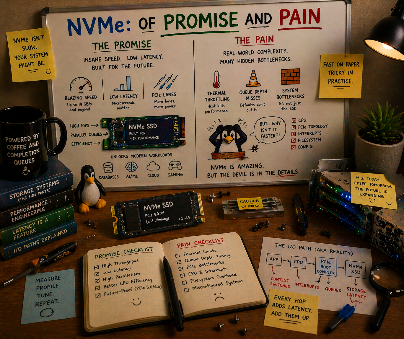
NVMe over Fabrics was supposed to make remote flash indistinguishable from local flash. Six years in, the reality is messier: TCP added latency that nobody budgeted for, RDMA requires a network engineering PhD, and half the industry is deploying NVMe-oF without understanding what they’re buying. Here’s what actually works, what quietly doesn’t, and what you should bet on for the next five years.
The Promise That Launched a Thousand Slides
The pitch was irresistible.
Local NVMe is fast: 10 microseconds for a 4KB random read, 7 GB/s sequential bandwidth on a single PCIe Gen4 x4 drive. But local NVMe has a problem: the drives are trapped inside the server. If Server A has idle flash capacity and Server B is starving for I/O, tough luck. You can’t share local NVMe across a network the way you share a SAN LUN or an NFS export.
NVMe over Fabrics, ratified by NVM Express in 2016, proposed the fix: extend the NVMe protocol over a network fabric so that remote drives appear as if they’re locally attached. Same NVMe command set. Same multi-queue architecture (65,535 queues, 65,536 commands each). Same sub-millisecond ambition. Just… over a wire instead of a PCIe bus.
The architecture diagrams wrote themselves:
┌─────────────────────────────────────────────┐
│            Compute Pool (Initiators)        │
│  ┌──────┐  ┌──────┐  ┌──────┐  ┌──────┐   │
│  │ GPU  │  │ GPU  │  │ GPU  │  │ GPU  │   │
│  │Node 1│  │Node 2│  │Node 3│  │Node N│   │
│  └──┬───┘  └──┬───┘  └──┬───┘  └──┬───┘   │
│     │         │         │         │        │
│ ════╪═════════╪═════════╪═════════╪══════  │
│     │     NVMe-oF Fabric (RDMA/TCP)        │
│ ════╪═════════╪═════════╪═════════╪══════  │
│     │         │         │         │        │
│  ┌──▼───┐  ┌──▼───┐  ┌──▼───┐  ┌──▼───┐   │
│  │Flash │  │Flash │  │Flash │  │Flash │   │
│  │JBOF 1│  │JBOF 2│  │JBOF 3│  │JBOF M│   │
│  │24xSSD│  │24xSSD│  │24xSSD│  │24xSSD│   │
│  └──────┘  └──────┘  └──────┘  └──────┘   │
│             Storage Pool (Targets)          │
└─────────────────────────────────────────────┘
Compute and storage scale independently. Any GPU node can access any flash shelf. Add more GPUs without adding more storage, or vice versa. This is disaggregation: the architectural pattern that every infrastructure vendor has been promising since 2018.
The promise: less than 10 microseconds of additional latency over RDMA. Remote NVMe that “feels local.”
Here’s what actually happened.
The Three Transports: A Tale of Trade-offs
NVMe-oF is not one protocol. It’s a command set that runs over multiple transports, and the transport you choose determines whether you get the promise or the pain.
Transport 1: RDMA (RoCEv2 and InfiniBand)
RDMA (Remote Direct Memory Access) lets one machine read from or write to another machine’s memory without involving either CPU. No kernel, no socket buffer copies, no TCP stack. Data moves directly from NIC to application memory via hardware-managed queue pairs.
The performance is real. RDMA over InfiniBand adds 2-5 microseconds to an NVMe I/O. RoCEv2 (RDMA over Converged Ethernet) adds 5-10 microseconds. At these latencies, remote NVMe genuinely starts to feel local. A 4KB random read that takes 10us locally takes 15us over RoCEv2. That’s a 50% latency increase on paper, but in absolute terms, 15 microseconds is still screaming fast.
InfiniBand is the simpler path. It’s a dedicated fabric: InfiniBand switches, InfiniBand HCAs (Host Channel Adapters), InfiniBand cables. The network is purpose-built for RDMA and has been doing it reliably since the early 2000s. NVIDIA’s ConnectX adapters and Quantum switches dominate this market. In HPC and AI clusters, InfiniBand is already there for GPU-to-GPU communication, so extending it to storage is natural.
Latency is exceptional. Bandwidth is exceptional. The catch is that you need a separate network. InfiniBand doesn’t converge with your Ethernet management network, your out-of-band network, or anything else. It’s a parallel universe of cabling and switching.
RoCEv2 tries to get InfiniBand’s performance on Ethernet infrastructure. Same RDMA semantics, same ConnectX adapters, but over standard Ethernet switches. This is where the pain begins.
RDMA assumes a lossless fabric. Drop a single packet and the RDMA connection stalls or resets. Unlike TCP, which gracefully retransmits, RDMA has no tolerance for loss. Ethernet, by design, drops packets when congested. To make RoCEv2 work, you need:
-
PFC (Priority Flow Control): Per-priority pause frames that prevent buffer overflow. Sounds great. In practice, PFC creates head-of-line blocking, pause storms that cascade across switches, and deadlocks in networks with cycles. Arista, Cisco, and Mellanox have all published white papers on how to configure PFC correctly. The fact that these white papers exist, and that they’re 40+ pages long, tells you everything about the difficulty.
-
ECN (Explicit Congestion Notification): Marks packets when queues build up, so senders can back off before drops occur. Requires ECN support on every switch in the path, correct threshold configuration, and a DCQCN (Data Center QCN) congestion control algorithm on the endpoints. Misconfigure the ECN marking threshold by 20% and you get either premature throttling (wasted bandwidth) or late marking (packet drops, RDMA failures).
-
DSCP-based QoS: Traffic classification to separate RDMA traffic from regular Ethernet traffic. Different queues, different priorities, different scheduling. On every switch. Consistently.
I’ve seen teams spend six months getting RoCEv2 stable on a 100-switch leaf-spine fabric. They hire a network consultant, reconfigure every switch, run ib_send_bw and ib_read_lat tests on every link, and eventually get it working. Then someone adds a new ToR switch with slightly different firmware and the pause storms return.
The dirty secret of RoCEv2: it works beautifully in controlled environments. A single rack with two leaf switches and homogeneous hardware? Flawless. A 500-node cluster with three tiers of switching from two vendors? Budget six months of network engineering and keep the consultant on retainer.
Transport 2: NVMe/TCP
NVMe/TCP, standardized in 2019 (TP8000), does the obvious thing: encapsulate NVMe commands in TCP segments and send them over standard Ethernet. No special NICs, no lossless fabric, no RDMA configuration. If you have an Ethernet network, you can run NVMe/TCP.
The latency reality:
| Operation | Local NVMe | NVMe/RDMA (RoCEv2) | NVMe/TCP | iSCSI |
|---|---|---|---|---|
| 4KB random read | ~10 us | ~15-20 us | ~40-80 us | ~100-200 us |
| 128KB sequential read | ~15 us | ~20-25 us | ~50-90 us | ~120-250 us |
| 4KB random write | ~15 us | ~20-30 us | ~50-100 us | ~150-300 us |
NVMe/TCP adds 30-80 microseconds of latency, depending on network conditions, CPU load, and how many TCP connections you’re multiplexing. That’s 3-8x the overhead of RDMA. “Feels local” it does not.
But here’s the thing: NVMe/TCP is still 2-5x faster than iSCSI, the protocol it replaces. And it runs on the network you already have. No PFC configuration. No lossless fabric. No network consultant. Install the nvme-tcp kernel module, point it at a target, and go.
For bulk data transfer (model checkpoint writes, dataset pre-staging, asynchronous replication), 50 microseconds of latency per I/O is perfectly acceptable. You’re streaming gigabytes; the throughput matters more than the per-I/O latency. At 100 GbE, NVMe/TCP saturates the link just fine.
Where NVMe/TCP breaks down:
The CPU cost. TCP processing is not free. Each NVMe/TCP connection consumes CPU cycles for segmentation, checksumming, and retransmission. At high IOPS (500K+), the host CPU spends significant cycles just running the TCP stack. This is precisely the overhead that RDMA eliminates.
Then there’s tail latency. TCP retransmission on packet loss adds milliseconds (the default RTO minimum is 200ms on Linux, though this can be tuned). RoCEv2 on a properly configured lossless fabric never retransmits; it pauses instead. For latency-sensitive workloads, a single TCP retransmission blows your P99.
TCP offload is changing the calculus. Modern NICs (ConnectX-7, Intel E810) offer NVMe/TCP hardware offload that moves the TCP state machine into the NIC firmware. Early benchmarks show offloaded NVMe/TCP approaching within 2x of RDMA latency at significantly reduced CPU consumption. This is the technology to watch. If NIC-offloaded NVMe/TCP can deliver 20-30us latency with near-zero CPU overhead, the case for RoCEv2’s complexity weakens considerably.
Transport 3: FC-NVMe
Fibre Channel NVMe runs NVMe commands over Fibre Channel fabrics. If you have an existing FC SAN infrastructure (many enterprises do, as banks, hospitals, and government agencies have invested millions), FC-NVMe lets you modernize the protocol without replacing the physical network.
The reality: FC-NVMe works well in existing FC environments. The latency is between RDMA and TCP (roughly 15-30us). The fabric management tools (Brocade FOS, Cisco MDS NX-OS) already handle zoning, multipath, and QoS. It’s a natural evolution for FC shops.
The trajectory: FC-NVMe is a bridge technology. New greenfield deployments overwhelmingly choose Ethernet (either RoCEv2 or TCP). FC-NVMe extends the life of existing FC investments, but FC’s market share has been declining for a decade and NVMe/TCP accelerates that decline. Gen7 FC at 64 Gb/s is competitive with 100 GbE today, but 400 GbE and 800 GbE are already shipping while FC Gen8 (128 Gb/s) is still in development.
Discovery, Multipath, and the Operational Reality
Choosing a transport is just the beginning. Once you have NVMe-oF connectivity, you need to solve three operational problems that don’t exist with local NVMe.
Discovery: How Do Initiators Find Targets?
Local NVMe is simple: the kernel scans the PCIe bus, finds NVMe controllers, creates /dev/nvmeXnY devices. Done.
NVMe-oF requires explicit discovery. The initiator must know where the targets are. Three mechanisms exist:
Static configuration. Hardcode target IP/port in /etc/nvme/discovery.conf or systemd unit files. Simple, brittle. Every time you add or move a storage target, you update every initiator’s config. This is how most deployments start, and how many still operate. It doesn’t scale past a few dozen nodes.
Discovery Controller. The NVMe spec defines a Discovery Controller service that initiators query to learn available subsystems and paths. The initiator connects to a well-known discovery endpoint, receives a list of (transport, address, subsystem NQN) tuples, and connects to the ones it needs. This is the right answer, but implementing a production-quality Discovery Controller requires handling registration, deregistration, health checks, access control, and multipath advertisement. Most open-source implementations are basic.
mDNS/DNS-SD. Draft spec for automatic discovery via multicast DNS. The “zero-configuration” dream. Not widely implemented yet, and multicast in large data center networks is a governance headache.
TP8009 (Centralized Discovery Controller). Ratified in 2022, CDC adds a persistent, centralized discovery service that can manage thousands of initiator-target relationships. Think of it as DNS for NVMe-oF. This is what production deployments need, but adoption is still early. Linux kernel support landed in 6.x, and SPDK has an implementation, but the ecosystem tooling (monitoring, RBAC, federation) is immature.
Multipath: Surviving Failures
In a local NVMe setup, the drive either works or it doesn’t. With NVMe-oF, the drive might be fine but the network path to it fails. Multipath means connecting to the same NVMe namespace through multiple independent network paths, so a single link or switch failure doesn’t cause an outage.
ANA (Asymmetric Namespace Access) is the NVMe spec’s answer. Each path to a namespace has an ANA state: Optimized, Non-Optimized, or Inaccessible. The host prefers Optimized paths and fails over to Non-Optimized paths when Optimized paths go down. This is analogous to ALUA (Asymmetric Logical Unit Access) in SCSI, and if you’ve configured ALUA multipath with multipathd, you know both the power and the misery.
Linux native multipath (nvme-core.multipath=Y kernel parameter) handles path selection in the kernel. It works. Failover times range from sub-second (when the failure is clean, like a TCP RST or an ANA state change notification) to 30+ seconds (when the failure is ambiguous, where a path goes silent and the transport timeout must expire before failover triggers).
The timeout problem. NVMe/TCP’s default ctrl-loss-tmo is 600 seconds. That means if a controller becomes unreachable, the host will retry for ten minutes before declaring the path dead. For many workloads, ten minutes of I/O stalls is indistinguishable from an outage. Tuning these timeouts (ctrl-loss-tmo, reconnect-delay, keep-alive-tmo, nr-io-queues) is an art that most deployment guides gloss over.
Here’s a set of timeouts that works for latency-sensitive workloads:
# /etc/nvme/discovery.conf or nvme connect parameters
--ctrl-loss-tmo=30       # give up after 30s, not 600s
--reconnect-delay=2      # retry every 2s, not 10s
--keep-alive-tmo=5       # detect controller death in 5s
--nr-io-queues=8         # match to CPU cores serving I/O
--nr-write-queues=4      # separate write queue pool
These values are aggressive. They trade resilience (a brief network hiccup triggers failover) for responsiveness (the application knows within seconds, not minutes). The right values depend on your tolerance for false positives.
Zoning and Security: The “See Everything” Problem
SAN administrators recognized this problem in 1999, and NVMe-oF is only now solving it.
By default, an NVMe-oF initiator that discovers a target can access every namespace on that target. There’s no isolation. In a multi-tenant environment, or even in a single-tenant environment where different teams own different storage pools, this is a security hole.
NVMe subsystem NQN-based access control is the basic mechanism: the target defines which initiator NQNs (NVMe Qualified Names) are allowed to connect to which subsystems. This is the equivalent of FC LUN masking, and it works, but it’s per-subsystem, not per-namespace. Fine-grained isolation requires one subsystem per tenant, which adds management overhead.
TLS 1.3 for NVMe/TCP (TP8011) adds encryption and authentication to the transport. Without it, NVMe/TCP traffic flows in cleartext, and any network tap sees your data. With TLS, you get encrypted transport plus certificate-based authentication. Linux kernel support is available as of 6.7, and SPDK added TLS support in 24.01. The performance impact is meaningful: expect 10-15% throughput reduction with software TLS, less with NIC-offloaded TLS.
In-band authentication (TP8010, DH-HMAC-CHAP) provides challenge-response authentication at the NVMe protocol level, independent of the transport. This matters for RDMA, where TLS isn’t applicable (RDMA bypasses the TCP stack entirely). DH-HMAC-CHAP with DH group negotiation provides reasonable security without transport-level encryption.
The honest assessment: NVMe-oF security in 2026 is roughly where iSCSI security was in 2008. It exists, it works, and almost nobody enables it because the performance cost feels unjustifiable in a trusted data center network. Then someone plugs a rogue device into the fabric and you have a very bad day.
What Works Today
Let’s be specific about where NVMe-oF is deployed in production and delivering value.
All-Flash Arrays
Pure Storage FlashArray, NetApp AFF, Dell PowerStore, and VAST Data all expose NVMe-oF front-end connectivity. These are traditional storage arrays that replaced FC-SCSI or iSCSI with NVMe-oF as the host-facing protocol.
Why it works: The array handles all the complexity. Discovery, multipath, namespace management, zoning: it’s all managed by the array’s control plane. The host just runs nvme connect and gets a block device. The operational model is identical to a traditional SAN, just faster.
The win: 2-5x IOPS improvement over iSCSI on the same hardware, with lower CPU utilization on the host. For database workloads (Oracle, SQL Server, PostgreSQL) that are latency-sensitive and IOPS-hungry, this is a genuine, measurable improvement.
NVIDIA DGX and AI Clusters
NVIDIA’s DGX SuperPOD reference architecture uses NVMe-oF (over InfiniBand) to connect GPU nodes to shared flash storage tiers. The BlueField DPU acts as both the NVMe-oF target (serving local NVMe drives to the fabric) and the initiator (consuming remote namespaces).
Why it works: InfiniBand is already there. DGX clusters run InfiniBand for NCCL (GPU-to-GPU communication), so extending it to storage adds no new infrastructure. BlueField handles NVMe-oF target/initiator duties in hardware, offloading the host CPU entirely. And NVIDIA controls the entire stack (DPU firmware, ConnectX drivers, DOCA SDK, Dynamo framework), so interoperability is tested by one vendor.
This is the most compelling NVMe-oF deployment model in 2026: AI clusters where InfiniBand is a given, BlueField handles the storage fabric, and the performance requirements (feeding 8x H100/B200 GPUs with training data) justify the infrastructure investment.
Hyperscaler Internal Infrastructure
AWS EBS, Google Persistent Disk, and Azure Managed Disk all use NVMe-oF internally to connect compute instances to remote storage. When you attach an EBS volume to an EC2 instance, the NVMe device you see in the guest is backed by NVMe-oF over the hyperscaler’s custom fabric.
Why it works: Hyperscalers control the switch firmware, the NIC firmware, the host kernel, and the storage backend. They can build lossless Ethernet fabrics with custom congestion control algorithms (AWS’s SRD, Google’s Snap) that wouldn’t work in a heterogeneous enterprise network. They can also deploy at a scale where the engineering investment amortizes to pennies per instance.
You can’t replicate this. But it’s worth knowing that NVMe-oF at scale does work, if you control every layer of the stack.
What Doesn’t Work (Yet)
General-Purpose Disaggregated Storage
The dream: separate compute and storage into independent pools. Scale each independently. Any compute node accesses any storage node over NVMe-oF.
Why it doesn’t work yet:
Tail latency. NVMe-oF adds a latency distribution, not a fixed overhead. The median is acceptable, but the P99 and P999 include TCP retransmissions, RDMA path failovers, and congestion events that add milliseconds. For workloads that are tolerant of tail latency (batch analytics, training data reads), this is fine. For workloads that aren’t (OLTP databases, real-time serving), it’s a deal-breaker.
Blast radius. A network partition in a disaggregated architecture can make storage inaccessible to every compute node simultaneously. With locally-attached storage, a network failure affects only network-dependent workloads, and local I/O continues. Full disaggregation means full dependency on the fabric.
Complexity cost. Running a disaggregated NVMe-oF fabric requires expertise in NVMe target management, fabric zoning, multipath configuration, timeout tuning, performance monitoring (which latencies are NVMe, which are fabric, which are congestion?), and capacity planning across the fabric. Most organizations don’t have this expertise, and the tooling to make it accessible doesn’t exist yet.
The organizations that successfully run disaggregated NVMe-oF in 2026 are hyperscalers and HPC centers with dedicated storage networking teams. Everybody else is doing DAS or hyper-converged.
Cross-Datacenter NVMe-oF
NVMe-oF over a WAN doesn’t work. The protocol was designed for data center fabrics with microsecond-scale RTTs. At 10ms WAN latency, the NVMe queuing model breaks down. You need thousands of outstanding commands to keep throughput high, but the NVMe/TCP connection stalls on flow control long before that.
Replication between data centers should use application-level protocols (HTTP, gRPC, custom replication streams), not NVMe-oF. This seems obvious, but I’ve seen it in vendor presentations: “NVMe-oF for DR replication.” No.
Multi-Tenant NVMe-oF Fabrics
Running multiple tenants on a shared NVMe-oF fabric requires per-tenant isolation (separate NQNs, access control, bandwidth guarantees), per-tenant QoS (one tenant’s sequential scan shouldn’t destroy another’s IOPS-sensitive workload), and per-tenant monitoring. The NVMe spec supports some of this (NVMe rate limiting, namespace-level QoS), but the tooling, orchestration, and operational practices are years behind what FC SANs offer.
Kubernetes persistent volumes over NVMe-oF (via the NVMe-oF CSI driver) are emerging, but they add another layer of abstraction on top of an already complex stack. Getting PV failover, resize, and snapshot operations working reliably through Kubernetes, CSI, NVMe-oF, and the target is a test of patience.
The Software Stack: Kernel vs. SPDK
NVMe-oF targets (the storage side) can run in-kernel or in user-space. The choice matters more than most people think.
Linux Kernel NVMe-oF Target (nvmet)
The kernel’s nvmet subsystem implements NVMe-oF targets using standard kernel block devices as backing stores. It’s included in mainline Linux, requires no additional software, and supports all three transports (RDMA, TCP, FC).
Pros: Simple to set up. Uses standard kernel block devices, so any filesystem, LVM, or device-mapper setup works as a backend. Integrates with kernel block layer features (QoS, cgroups, dm-crypt). Operational tools (nvmetcli, configfs) are straightforward.
Cons: Performance is limited by the kernel block layer overhead. At high IOPS (1M+), the CPU cost of crossing the kernel block layer for each I/O becomes significant. TCP transport performance is particularly affected, as both the NVMe target processing and TCP stack run in kernel context, competing for CPU.
Real-world performance: A single nvmet TCP target serving 8 NVMe drives can deliver roughly 600K-800K IOPS on a modern dual-socket server. For many workloads, this is plenty. For an all-flash array or a dedicated storage node serving a GPU cluster, it’s the bottleneck.
SPDK NVMe-oF Target
SPDK runs the NVMe-oF target entirely in user-space. NVMe drives are unbound from the kernel, and both the NVMe backend and the NVMe-oF transport (RDMA or TCP) run in polled mode on dedicated cores.
Pros: Performance. SPDK’s NVMe-oF target delivers 2-4x the IOPS of the kernel target at lower and more consistent latency. For TCP transport, SPDK uses its own user-space TCP stack (POSIX sockets or DPDK-based), avoiding the kernel TCP overhead.
Cons: Everything I described in the io_uring and SPDK piece. Dedicated cores, hugepage memory, no filesystem, no kernel tooling. The operational complexity is significant.
Who uses it: Storage vendors building NVMe-oF appliances (Lightbits, E8 Storage/VAST Data, Samsung SmartSSD), and hyperscalers running custom storage backends. If you’re building a storage product, SPDK makes sense. If you’re running a storage service on general-purpose infrastructure, the kernel target is the pragmatic choice.
The Middle Path: io_uring-Based Targets
The emerging third option is an NVMe-oF target built on io_uring for backend I/O with kernel TCP or RDMA for the fabric transport. This keeps the drives in kernel space (operational tooling works), uses io_uring’s async I/O for near-SPDK backend performance, and avoids SPDK’s dedicated-core requirement.
No production-ready open-source implementation exists yet, but this is the architectural direction that makes the most sense for software-defined storage projects. The kernel nvmet target is slowly gaining io_uring integration, and several startups are building user-space targets on io_uring.
The Ethernet Speed Ladder: When TCP Stops Losing
There’s a subtle dynamic that most NVMe-oF discussions miss: the latency gap between RDMA and TCP narrows as Ethernet speeds increase.
Here’s why. NVMe/TCP’s overhead has two components: protocol processing (serializing NVMe commands into TCP segments, checksumming, managing connections) and serialization delay (the time to put bits on the wire).
At 25 GbE, serializing a 4KB NVMe command + data payload takes about 1.3 microseconds. At 100 GbE, it takes 0.3 microseconds. At 400 GbE, it takes 0.08 microseconds. The serialization delay is shrinking toward zero.
Protocol processing overhead is relatively constant (a few microseconds for software TCP, sub-microsecond for NIC-offloaded TCP). As serialization delay becomes negligible, the gap between TCP and RDMA compresses to just the protocol processing difference.
| Ethernet Speed | NVMe/TCP 4KB Latency (sw) | NVMe/TCP 4KB Latency (offload) | NVMe/RDMA 4KB Latency |
|---|---|---|---|
| 25 GbE | ~60-80 us | ~35-50 us | ~10-15 us |
| 100 GbE | ~40-60 us | ~20-35 us | ~8-12 us |
| 200 GbE | ~30-50 us | ~15-25 us | ~7-10 us |
| 400 GbE | ~25-40 us | ~10-20 us | ~5-8 us |
At 400 GbE with TCP offload, the gap between TCP and RDMA is 2x or less. Still measurable, but for bulk transfer workloads (streaming training data, checkpoint writes, replication), the difference is academic. You save the six months of lossless Ethernet configuration and the network consultant’s fees.
This is why I believe NVMe/TCP with NIC offload will be the dominant NVMe-oF transport by 2028 for all workloads except ultra-low-latency database access. RDMA will remain important for InfiniBand-based AI clusters where it’s already deployed, but new Ethernet-based deployments will increasingly choose TCP + offload over the operational burden of RoCEv2.
CXL vs. NVMe-oF: Complementary, Not Competing
A question I hear frequently: “Does CXL replace NVMe-oF?”
No. They operate at different scales and different latency tiers.
CXL (Compute Express Link) is a PCIe-based coherency protocol designed for rack-scale interconnect. CXL 3.0 supports fabric switching, but the target distance is short: meters, not hundreds of meters. CXL latency for memory access is 150-300 nanoseconds, an order of magnitude faster than NVMe-oF. CXL is for sharing memory and metadata within a rack or a few racks connected by a CXL switch fabric.
NVMe-oF operates at pod and cluster scale: tens to hundreds of meters over Ethernet or InfiniBand. Latency is microseconds to tens of microseconds. NVMe-oF is for accessing storage across a data center.
The architecture that emerges combines both:
┌─────────────────────────────────────┐
│          Within a Rack              │
│  CXL 3.0 fabric: 150-300ns         │
│  Shared metadata, pooled memory     │
│  Cache-coherent access across hosts │
├─────────────────────────────────────┤
│          Within a Pod (10-100m)     │
│  NVMe-oF RDMA: 5-15us              │
│  Disaggregated flash access         │
│  Shared storage pools               │
├─────────────────────────────────────┤
│          Within a DC (100m-2km)     │
│  NVMe/TCP: 30-80us                 │
│  Bulk data transfer, replication    │
│  Tiered storage access              │
├─────────────────────────────────────┤
│          Across DCs (WAN)           │
│  HTTP/S3: milliseconds             │
│  Replication, DR, cross-region      │
│  Object storage as durable tier     │
└─────────────────────────────────────┘
Each protocol owns a latency tier and a distance budget. Trying to stretch any one of them outside its tier produces misery: CXL across a data center doesn’t work (distance), NVMe-oF across a WAN doesn’t work (latency), and S3 for low-latency local access doesn’t work (overhead).
The storage software that wins is the one that speaks all four tiers and places data in the right one based on access patterns. Model weights that haven’t been accessed in a week live in S3 (object storage). Model weights being loaded for inference pre-stage via NVMe-oF to a local JBOF. KV cache metadata is coordinated via CXL shared memory. Active KV cache lives in GPU HBM. Each tier serves its purpose.
What Storage Software Needs to Change
Most storage software was designed for either local disks or TCP-based network protocols (NFS, iSCSI, S3). NVMe-oF introduces requirements that break assumptions baked into every layer.
Connection Management
A traditional NFS client maintains one or a few TCP connections to a server. An iSCSI initiator manages a small number of sessions. NVMe-oF, by contrast, creates multiple I/O queues per connection (typically one per CPU core), and each queue can have thousands of outstanding commands.
Storage software needs to manage these queue resources explicitly: allocating the right number of I/O queues based on workload, monitoring per-queue depth and latency, and rebalancing when paths change. Over-allocating queues wastes target resources. Under-allocating leaves performance on the table.
NUMA-Aware Path Placement
On a dual-socket server, NVMe-oF connections land on a specific NIC, which is attached to a specific PCIe root complex, which is local to a specific NUMA node. If the application thread processing I/O completions runs on the other NUMA node, every completion incurs a cross-socket memory access (an extra 100-200 nanoseconds per I/O). For a deeper dive into PCIe topology and NUMA effects on storage, see the PCIe lanes and NUMA-aware storage post.
At local NVMe speeds, this doesn’t matter much. At NVMe-oF speeds, where you’re fighting for every microsecond, cross-NUMA completions can add 10-15% latency. Storage software should pin NVMe-oF I/O processing to cores on the same NUMA node as the NIC.
Timeout Tuning
As discussed above, default NVMe-oF timeouts are conservative (600 seconds for controller loss). Storage software that builds on NVMe-oF must expose and intelligently manage these timeouts, because the right values depend on the workload’s tolerance for stalls versus false failovers.
For AI training workloads (where a 30-second I/O stall means wasted GPU-hours at thousands of dollars per hour), aggressive timeouts with fast failover are essential. For database workloads (where a false failover can cause split-brain or data corruption), conservative timeouts are safer.
Performance Monitoring
“The storage is slow” is no longer a simple diagnosis. With NVMe-oF, latency has three components:
- Target-side device latency. The NVMe drive itself. Usually 10-20us for reads.
- Fabric latency. Network transit time, including serialization, switching, and any congestion. Depends on transport (5us for RDMA, 30-80us for TCP).
- Host-side processing latency. Kernel or SPDK command processing, memory copies, interrupt handling.
Diagnosing a latency regression requires decomposing total latency into these components. NVMe-oF provides some help: the NVMe-oF target can stamp commands with target-side completion time, and the host can measure round-trip time. The difference is fabric + host processing. But standard monitoring tools (iostat, blktrace) don’t distinguish these components, and most storage observability stacks need new instrumentation.
What to Bet On
If you’re making NVMe-oF decisions in 2026, here’s the practical guidance:
If you already have InfiniBand (AI/HPC clusters): Use NVMe-oF over InfiniBand. You have the fabric, the NICs, and the expertise. Add NVMe-oF targets to your existing fabric. This is the lowest-risk, highest-performance option.
If you’re building new Ethernet infrastructure: Start with NVMe/TCP. Get it working, get it monitored, get your timeout tuning right. Plan for NIC-offloaded TCP as the performance upgrade path. Only invest in RoCEv2 if you have a specific latency requirement that TCP can’t meet AND you have the network engineering team to maintain a lossless fabric.
If you have an existing FC SAN: FC-NVMe is a natural upgrade. Same fabric, faster protocol. Don’t rip out FC to build an Ethernet NVMe-oF fabric unless you have a compelling reason beyond protocol modernization.
If you’re building storage software: Abstract the transport. Your storage engine should not care whether the backend is local NVMe, NVMe-oF over RDMA, NVMe-oF over TCP, or a remote S3 endpoint. Use an IoEngine trait (or equivalent) that abstracts read/write/trim operations, and let deployment configuration choose the transport. Test against all of them. Your users’ infrastructure is heterogeneous even if yours isn’t.
If you’re evaluating disaggregation: Be skeptical. The architecture diagrams are beautiful, but the operational reality is 10x more complex than DAS or hyper-converged. Start with a single-rack proof of concept. Measure tail latency, not just median latency. Test failure scenarios: what happens when a switch goes down, when a path flaps, when a target reboots during heavy I/O? If the answers are acceptable, scale cautiously.
The Honest Summary
NVMe-oF is real infrastructure solving real problems. It’s not vaporware, and it’s not just benchmarks. All-flash arrays with NVMe-oF front ends are measurably faster than iSCSI. AI clusters with InfiniBand NVMe-oF are feeding GPUs effectively. Hyperscalers run their entire block storage stack on NVMe-oF at billions of IOPS.
But the gap between “NVMe-oF works” and “NVMe-oF feels local” is still wide for most organizations. TCP adds real latency. RDMA adds real complexity. Discovery and multipath tooling is immature. Security is an afterthought. And the operational expertise required to run a production NVMe-oF fabric is significantly higher than what most teams have.
The trajectory is positive. NIC-offloaded TCP is narrowing the RDMA gap. Centralized discovery controllers are maturing. The kernel NVMe-oF stack improves with every release. Five years from now, NVMe-oF over TCP will be as unremarkable as iSCSI is today, standard infrastructure that just works.
But we’re not there yet. In 2026, NVMe-oF is a technology that rewards expertise and punishes assumptions. The promise is real. The pain is real too. The winners are the teams that understand both.
NVMe-oF specifications are maintained by NVM Express, Inc. NVMe-oF transport specs: TP8000 (TCP), TP8010 (In-Band Authentication), TP8011 (TLS), TP8009 (Centralized Discovery Controller). Linux kernel NVMe-oF documentation at kernel.org. SPDK NVMe-oF target documentation at spdk.io. SNIA NVMe-oF interoperability testing conducted at SNIA Plugfest events. NVIDIA BlueField DPU NVMe-oF capabilities at NVIDIA DOCA documentation. Latency measurements cited from VU Amsterdam CHEOPS ‘23, Samsung PM9A3 data sheets, and published NVMe/TCP benchmarks from Lightbits Labs and Samsung.
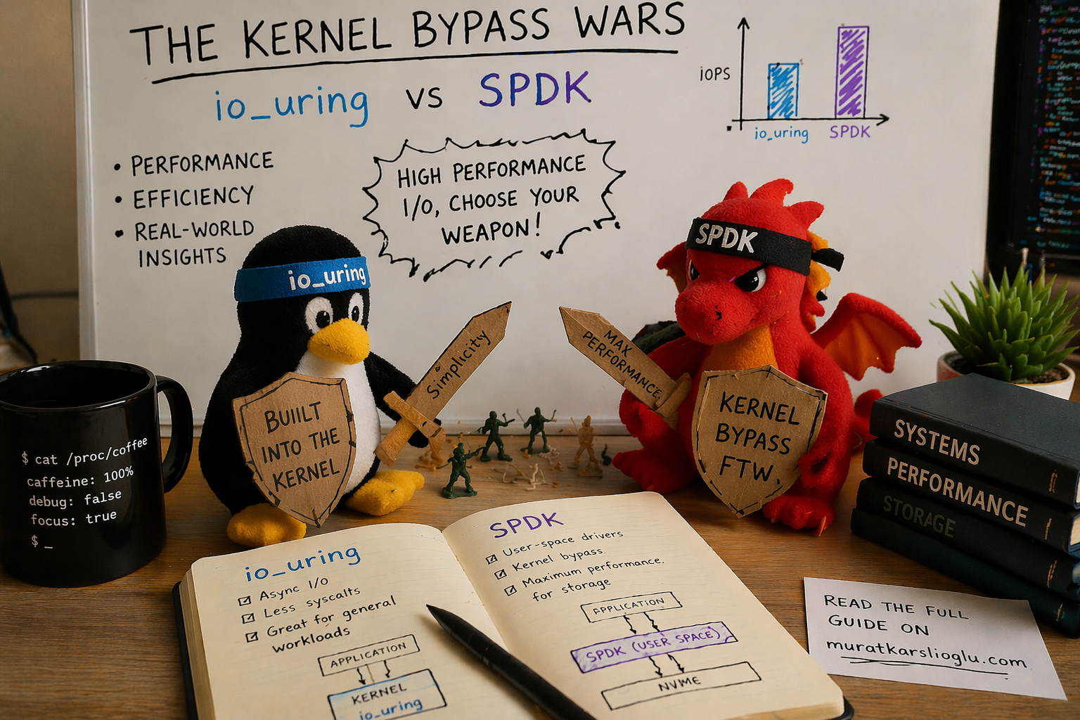
The Linux kernel I/O stack was designed when a disk seek took 10 milliseconds. NVMe completes I/O in 10 microseconds. The kernel overhead (context switches, VFS traversal, page cache, block layer, scheduler) now consumes 40% of your I/O latency. Two approaches emerged to fix this: SPDK (rip out the kernel entirely) and io_uring (make the kernel fast enough that you don’t need to). SPDK won the benchmarks. io_uring is winning the war. Here’s why.
The Syscall Tax: Why the Kernel Is the Bottleneck
Every traditional Linux I/O operation follows the same path:
Application                          Kernel
    │                                   │
    ├─ read() ──── context switch ────► VFS layer
    │                                   ├─► page cache lookup
    │                                   ├─► filesystem (ext4/XFS)
    │                                   ├─► block layer (bio, elevator)
    │                                   ├─► NVMe driver
    │                                   ├─► device interrupt
    │                                   ├─► completion processing
    ◄── context switch ────────────────┘
    │
    ├─ ~4 microseconds overhead
Each read() or write() crosses the user-kernel boundary twice, walks the VFS, checks the page cache, traverses the block layer, and wakes the thread on completion via interrupt. On a good day, the overhead is about 4 microseconds per I/O.
When the storage device was a spinning disk with a 10ms seek time, 4us of kernel overhead was 0.04%. Invisible. Free.
A modern NVMe SSD completes a 4KB random read in about 10 microseconds. Now that 4us kernel overhead is 40% of your total I/O latency. The kernel isn’t managing the device anymore. It’s competing with it.
At scale, this gets worse. A single Samsung PM9A3 NVMe drive handles 900K random read IOPS. At 24 drives per node, that’s 21.6 million potential IOPS. Each IOP requires at least one syscall, one context switch, one interrupt. The CPU spends more time managing I/O than the drives spend doing I/O.
This is why the storage industry went looking for alternatives.
SPDK: The Nuclear Option
Intel’s Storage Performance Development Kit (SPDK) takes the most aggressive possible approach: remove the kernel from the I/O path entirely. NVMe devices are unbound from the Linux kernel driver, bound to a user-space driver (via VFIO or UIO), and the application talks directly to the NVMe submission and completion queues through memory-mapped registers.
No syscalls. No context switches. No VFS. No block layer. No interrupts. The application polls the completion queue in a tight loop, burning CPU cycles to achieve the lowest possible latency.
The performance is real. Research from VU Amsterdam (CHEOPS ‘23, SYSTOR ‘22) measured SPDK delivering 4.2 million IOPS using only 5 CPU cores, peak throughput that no other I/O API could match. At low queue depths where latency matters most, SPDK’s polled completion eliminates the interrupt latency that penalizes every other approach.
What SPDK Costs You
But SPDK doesn’t just bypass the kernel’s I/O stack. It bypasses the kernel’s everything:
Hugepages. SPDK requires pre-allocated hugepages, minimum 2 GB, pinned in physical memory before the application starts. The memory must be physically contiguous for DMA, which means you’re reserving large chunks of RAM at boot time. Memory fragmentation on long-running systems makes this increasingly unreliable. GitHub issue #707 documents production systems failing to allocate hugepages after weeks of uptime.
Dedicated CPU cores. SPDK runs in polled mode, consuming 100% of each dedicated core. Research from HotStorage ‘25 (“SPDK+: Low Latency or High Power Efficiency?”) measured that when polling 7 NVMe drives at queue depth 8, only 15.17% of clock cycles were actively used. The remaining 84.83% are wasted spinning on an empty completion queue. You’re paying for 6 CPU cores to get the useful work of 1.
Device unbinding. NVMe devices must be unbound from the kernel’s nvme driver and rebound to vfio-pci or uio_pci_generic via SPDK’s setup.sh script. While SPDK owns a device, it’s invisible to the operating system. No lsblk. No smartctl. No filesystem. No kernel QoS, no cgroups, no quota enforcement. Your operational tooling goes dark.
Custom memory management. All data buffers must be allocated via spdk_dma_malloc() for DMA-safe, physically-pinned memory. Standard malloc() buffers cannot be used for I/O. Every library, every abstraction layer, every buffer pool in your application must be aware of this constraint.
DPDK dependency. SPDK depends on Intel’s Data Plane Development Kit (DPDK) for memory management and device infrastructure. DPDK is itself a large, complex C library with its own hugepage requirements, EAL (Environment Abstraction Layer) initialization, and threading model. You’re not just adopting SPDK. You’re adopting SPDK and DPDK.
No filesystem integration. This is the one that kills most adoption attempts. With SPDK, there is no filesystem on top of the NVMe device. No ext4, no XFS, no file permissions, no ls, no dd, no cp. You get raw block access. Building anything on top (an object store, a database, a log-structured storage engine) means implementing your own space management, your own allocation, your own crash recovery. From scratch.
The SPDK Adoption Picture
Given all of this, SPDK’s production footprint is concentrated in a few categories:
-
Purpose-built storage appliances: VAST Data uses SPDK in their metadata path, reporting 30-40% better latency and 50-100% IOPS improvement. Nutanix’s Acropolis BlockStore is built entirely on SPDK. These are teams with 50-100 storage engineers dedicated to a single product.
-
NVMe-oF targets: OpenEBS/Mayastor uses SPDK to expose Kubernetes persistent volumes over NVMe over Fabrics. Longhorn V2 (SUSE) has an experimental SPDK data engine. Both require a full CPU core per node and kernel 6.7+.
-
Hardware vendors: Samsung and Intel are major SPDK contributors, using it internally for firmware validation and performance testing.
Notice who’s missing? General-purpose storage systems. Databases. Application developers. The teams that build 90% of the world’s storage software. For them, SPDK’s operational burden (hugepages, dedicated cores, device unbinding, custom allocators, no filesystem) is a price they can’t or won’t pay.
The industry needed something between “4us of kernel overhead on every I/O” and “rip out the entire kernel.” That something is io_uring.
io_uring: Making the Kernel Fast Enough
io_uring, introduced by Jens Axboe in Linux 5.1 (May 2019), takes a fundamentally different approach than SPDK. Instead of bypassing the kernel, it redesigns how applications talk to the kernel.
The core insight: the expensive part of a syscall isn’t the work, it’s the transition. Crossing from user space to kernel space and back costs 100-500ns per call due to context switching, TLB flushes, and speculative execution mitigations (KPTI, Spectre). If you could submit a batch of I/O operations without a syscall per operation, and harvest completions without a syscall per completion, the overhead drops by an order of magnitude.
The Ring Buffer Architecture
io_uring uses two shared memory ring buffers: a Submission Queue (SQ) and a Completion Queue (CQ), mapped into both user space and kernel space.
User Space                         Kernel Space
    │                                   │
    ├─ Write SQE to SQ ring ───────────►│ (no syscall, just memory write)
    ├─ Write SQE to SQ ring ───────────►│
    ├─ Write SQE to SQ ring ───────────►│
    ├─ io_uring_enter() ───────────────►│  (one syscall, submits all 3)
    │                                   ├─► process I/O operations
    │                                   ├─► write CQEs to CQ ring
    ◄── read CQE from CQ ring ─────────┤ (no syscall, just memory read)
    ◄── read CQE from CQ ring ─────────┤
    ◄── read CQE from CQ ring ─────────┤
The application writes Submission Queue Entries (SQEs) directly into the shared ring, no syscall needed. When it’s ready, a single io_uring_enter() call submits the entire batch to the kernel. Completions appear in the CQ ring, readable from user space without any syscall.
One syscall for N operations, versus N syscalls for N operations with read()/write().
The Evolution: 2019 to 2026
io_uring didn’t ship fully formed. It evolved over 30+ kernel releases, each adding capabilities that closed the gap with SPDK:
| Kernel | Year | Capability | Impact |
|---|---|---|---|
| 5.1 | 2019 | Basic SQ/CQ rings | Foundation: batched async I/O |
| 5.3 | 2019 | Linked SQEs | Dependent I/O chains without round-trips |
| 5.6 | 2020 | Fixed files, 30 opcodes | Eliminate fd refcount overhead |
| 5.7 | 2020 | Internal polling (FAST_POLL) | Eliminate async thread punt |
| 5.11 | 2021 | Unprivileged SQPOLL | Kernel-side submission thread, no syscall at all |
| 5.19 | 2022 | io_uring_cmd (NVMe passthrough) | Bypass block layer entirely |
| 6.0 | 2022 | Zero-copy network send, ublk | Network I/O, user-space block drivers |
| 6.10 | 2024 | Improved zerocopy, bundles | 3x fewer cycles per byte for networking |
| 6.12 | 2024 | Hugepage coalescing, async discard | 5-6x faster discard, less CPU |
Two features deserve special attention.
SQPOLL: Eliminating the Last Syscall
With IORING_SETUP_SQPOLL, the kernel spawns a dedicated thread that polls the submission queue. The application writes SQEs to the ring and the kernel thread picks them up. Zero syscalls on the submission path. Completions are read from the CQ ring, also without a syscall. The entire I/O path becomes shared-memory communication between the application and a kernel thread.
This is architecturally identical to SPDK’s approach (poll-based, no interrupts) but with the kernel still managing the device. You keep your filesystem, your smartctl, your cgroups, your permission model. The NVMe device stays visible to the OS.
The cost is one kernel thread burning a CPU core, the same cost as SPDK’s poll loop, but with the kernel’s infrastructure intact.
io_uring_cmd: NVMe Passthrough Without SPDK
Added in kernel 5.19, io_uring_cmd (also called NVMe passthrough) lets applications submit native NVMe commands directly to device queues via io_uring, bypassing the entire Linux block layer (bio allocation, I/O scheduler, merge logic) while still going through the kernel’s NVMe driver.
Traditional path:     app → syscall → VFS → filesystem → block layer → NVMe driver → device
io_uring path:        app → SQ ring → block layer → NVMe driver → device
io_uring_cmd path:    app → SQ ring → NVMe driver → device
The results, measured at USENIX FAST ‘24 by the Samsung/Western Digital team:
- Block I/O path: up to 2.9 million IOPS
- io_uring_cmd passthrough: up to 3.9 million IOPS, a 35% improvement
- Combined with fixed buffers and polling: within 9-16% of raw SPDK performance
That’s SPDK territory. Without hugepages, without device unbinding, without custom allocators, without losing your filesystem, without DPDK. The device stays in the kernel’s NVMe driver. You can still run smartctl. You can still use cgroups. You can still see the device in lsblk.
io_uring_cmd is integrated into fio (--ioengine=io_uring_cmd --cmd_type=nvme) and into xNVMe, Samsung’s cross-platform NVMe access library. It’s the closest thing to “SPDK performance with kernel manners.”
The Numbers: io_uring vs SPDK in 2026
Let me lay out the performance data honestly. SPDK is still faster. The question is whether the gap justifies the cost.
Raw IOPS (Single NVMe, 4K Random Read)
| Configuration | IOPS | CPU Cores Used |
|---|---|---|
read() synchronous | ~15K (QD1) | 1 |
| libaio | ~600K | 1-2 |
| io_uring (interrupt) | ~850K | 1-2 |
| io_uring (SQPOLL) | ~950K | 2 (1 app + 1 kernel poll) |
| io_uring_cmd (passthrough + poll) | ~1.3M | 2 |
| SPDK (polled) | ~1.5M | 1-2 (dedicated) |
Source: fio benchmarks, FAST ‘24, CHEOPS ‘23.
Multi-Drive Aggregate (8x PCIe 5.0 NVMe)
From the December 2024 DBMS benchmark (8x Kioxia CM7-R, 2.45M IOPS per drive):
| Configuration | Aggregate IOPS | Notes |
|---|---|---|
| Synchronous | ~100K | Pathetic |
| io_uring (basic) | ~1.1M | Good baseline |
| io_uring + registered buffers | ~1.4M | 11% gain from buffer pre-registration |
| io_uring_cmd + IOPoll | ~2.3M | Block layer bypass |
| io_uring + SQPOLL (full stack) | ~3.3M | Peak io_uring config |
| SPDK | ~4.2M | Peak, 5 dedicated cores |
io_uring with the full optimization stack (SQPOLL + io_uring_cmd + registered buffers + fixed files) reaches ~80% of SPDK’s peak IOPS while retaining full kernel integration. For database workloads (PostgreSQL), applying io_uring optimization guidelines yielded a 14% throughput improvement over baseline. Meaningful, not revolutionary, but free.
The Real Comparison
The fair comparison isn’t “io_uring peak IOPS vs SPDK peak IOPS.” It’s:
| io_uring (full optimization) | SPDK | |
|---|---|---|
| Peak IOPS | ~80% of SPDK | 100% (reference) |
| CPU efficiency | Comparable with SQPOLL | 84% wasted cycles polling |
| Kernel integration | Full (cgroups, permissions, fs) | None |
| Device visibility | lsblk, smartctl, everything | Invisible to OS |
| Memory management | Standard malloc() + registered buffers | spdk_dma_malloc() only |
| Hugepages | Not required | Required (2GB+ pre-allocated) |
| Dependencies | Linux kernel 5.19+ | SPDK + DPDK + vfio/uio |
| Filesystem support | ext4, XFS, anything | None, raw block only |
| Operational tooling | All standard Linux tools | Custom tooling required |
| Build complexity | #include <liburing.h> | Link SPDK + DPDK + configure EAL |
You’re trading 20% peak IOPS for an operational cost reduction that’s hard to overstate. And that 20% gap continues to shrink with every kernel release.
The Security Elephant
I would be dishonest if I didn’t address io_uring’s security record. It’s bad.
The CVE Count
| Year | io_uring CVEs |
|---|---|
| 2021 | ~10 |
| 2022 | ~15 |
| 2023 | ~19 |
| 2024 | ~21 |
| 2025 | ~10 (partial year) |
That’s approximately 75 CVEs in 5 years for a single kernel subsystem. For context, the entire NVMe driver has had a handful in the same period.
The Highlights Reel
- CVE-2021-41073: Type confusion leading to local privilege escalation. Public exploit on GitHub.
- CVE-2022-29582: Use-after-free, cross-cache exploit. Full LPE writeup published.
- CVE-2024-0582: Use-after-free in provided buffer rings. Patched in mainline December 2023, but not ported to Ubuntu for two months, a patch gap exploited in the wild.
The Google Verdict
In June 2023, Google reported that 60% of kernel exploits submitted to their bug bounty in 2022 targeted io_uring. They paid out roughly $1 million in io_uring vulnerability rewards. Their response was sweeping:
- ChromeOS: io_uring disabled entirely
- Android: seccomp-bpf blocks io_uring for apps
- Google production servers: io_uring disabled
When Google, which runs one of the largest storage infrastructures on Earth, disables a feature, the storage industry should pay attention.
The Curing Rootkit
In April 2025, security firm ARMO published a proof-of-concept rootkit called “Curing” that operates entirely via io_uring’s 61 supported operations. Because io_uring operations don’t go through the syscall path, they completely bypass syscall-based security monitoring. Tested tools that failed to detect it: Falco, Microsoft Defender, and most Linux runtime security tools.
The mitigation requires KRSI (Kernel Runtime Security Instrumentation) using eBPF programs attached to LSM hooks, a capability that most production security stacks don’t have yet.
The Container Situation
- Docker 25.0.0+ (January 2024): io_uring blocked by default seccomp profile
- containerd: Runtime default seccomp profile updated to block io_uring
- Podman: Community discussions on the same restrictions
If you’re running storage in containers (Kubernetes), you need to explicitly allow io_uring syscalls in your seccomp profile. This is a deliberate decision with security trade-offs, not something you should do casually.
What This Means in Practice
For storage systems that run on dedicated bare-metal nodes (which most serious storage deployments do), io_uring’s security profile is manageable. You control the kernel, the seccomp policy, the attack surface. The CVEs are local privilege escalation; they require existing code execution on the machine. A storage appliance that only runs trusted storage software has a small attack surface regardless.
For storage running in multi-tenant containers or shared cloud VMs, io_uring’s security posture is a real concern. The default seccomp restrictions exist for good reason. You’re adding kernel attack surface for I/O performance that may or may not be your bottleneck.
The honest engineering answer: use io_uring on dedicated storage nodes where you control the stack. Fall back to libaio (or regular io_uring without SQPOLL/passthrough) in restricted environments. Test your security tooling against Curing-style attacks before assuming your monitoring covers io_uring operations.
Rust and io_uring: The Ecosystem Reality
Rust is the natural language for io_uring storage systems. No GC to interfere with I/O-pinned threads, no runtime to fight with. But the Rust io_uring ecosystem is fragmented in a way that matters for architectural decisions.
The Foundation: io-uring Crate
The low-level io-uring crate (34 million downloads, actively maintained under the tokio-rs organization) provides safe Rust bindings to liburing. It’s solid, well-tested, and the foundation that everything else builds on. If you’re building a storage engine and want direct control over SQE/CQE management, this is the right starting point.
The Runtime Layer: Three Competing Models
tokio-uring (tokio-rs): The official Tokio io_uring integration. Semi-dormant; last release May 2024, many open issues. It runs an io_uring event loop alongside Tokio’s epoll-based reactor, which means you get io_uring for file I/O but still use epoll for networking. Not production-ready by community consensus.
glommio (Datadog): Thread-per-core design, cooperative scheduling, direct io_uring usage without Tokio. Actively maintained. Used at Datadog for high-throughput data pipeline components. Linux-only, no cross-platform story. The most mature option for server-side Rust io_uring.
monoio (ByteDance): Thread-per-core, pure io_uring/epoll runtime. Used in production at ByteDance via the Monolake framework for application gateways. Benchmarks show peak performance close to 3x Tokio under 16 cores. Most performant of the three, and provides cancellable I/O components that address the fundamental safety issue.
The Cancellation Problem
There’s a fundamental tension between Rust’s async model and io_uring. When you drop an async future in Rust, the language guarantees the computation stops. But io_uring operations are submitted to the kernel. Dropping the future doesn’t cancel the kernel-side I/O. The kernel may still be writing to your buffer after Rust has freed it.
Standard Rust async I/O uses borrowed buffers:
async fn read(&mut self, buf: &mut [u8]) -> io::Result<usize>This is unsound with io_uring. If the future is dropped while the kernel is writing to buf, you have a use-after-free. All io_uring runtimes must instead use buffer-ownership semantics:
async fn read(buf: Vec<u8>) -> (io::Result<usize>, Vec<u8>)The buffer is moved into the future, and returned alongside the result. The kernel can write to it safely because the buffer’s lifetime is tied to the operation, not to a borrow.
This means io_uring-based Rust code is not API-compatible with the standard tokio::io::AsyncRead/AsyncWrite traits. Libraries built for Tokio’s epoll model don’t work with io_uring runtimes without adaptation. This is the single biggest obstacle to io_uring adoption in the Rust ecosystem.
The Practical Recommendation
For a storage system in 2026:
- Use the
io-uringcrate directly for the I/O engine, with your own SQE/CQE management. You want fine-grained control over submission batching, registered buffers, and polling mode anyway. - Use Tokio for everything else: networking, timers, task scheduling, the S3 HTTP layer.
- Bridge the two with a dedicated I/O thread pool that owns the io_uring instances and communicates with Tokio tasks via channels. This is the same architecture that ScyllaDB’s Seastar uses (separate I/O reactor, separate network reactor), adapted for Rust.
Don’t wait for tokio-uring to mature. Don’t rewrite your network stack on glommio or monoio. Use io_uring where it matters (disk I/O) and Tokio where it’s proven (everything else).
The Middle Path: What Actually Makes Sense
The storage industry’s io_uring vs SPDK debate is a false dichotomy. The right architecture uses io_uring differently for different parts of the I/O stack.
For Bulk Data I/O: io_uring with Direct I/O
Object storage is sequential-write, random-read. For bulk data operations (PUT shards to disk, GET shards from disk), io_uring with O_DIRECT and registered buffers eliminates both the page cache (which you don’t want for object storage, since you have your own caching) and the per-I/O buffer mapping overhead.
PUT shard pipeline:
    Compress → Encrypt → EC Encode → io_uring O_DIRECT write (batched, registered buffers)

GET shard pipeline:
    io_uring O_DIRECT read (batched, registered buffers) → EC Decode → Decrypt → Decompress
Multiple shard writes from a single PUT can be batched into a single io_uring_enter() call. For a 12-shard erasure coded write, that’s 12 I/O operations submitted with one syscall instead of 12.
For Metadata I/O: io_uring with Buffered I/O
Metadata files (FlatBuffer shard metadata, listing caches, bucket configs) are small, frequently accessed, and benefit from the page cache. Regular io_uring (not O_DIRECT) lets the kernel cache hot metadata in memory while still batching submissions.
For NVMe-Dense Nodes: io_uring_cmd Passthrough
On dedicated storage nodes with 24-48 NVMe drives, io_uring_cmd passthrough eliminates the block layer overhead entirely. You’re talking directly to the NVMe driver, skipping bio allocation, I/O scheduling, and merge logic. This is where io_uring approaches SPDK performance.
The requirement: kernel 5.19+ and using the NVMe character device (/dev/ngXnY) instead of the block device (/dev/nvmeXnYpZ). The drives remain visible to the kernel, but I/O bypasses the generic block layer.
For Networking: Tokio (epoll), Not io_uring
io_uring’s networking support is improving (zero-copy send in 6.0, zero-copy receive in 6.17), but epoll-based networking is battle-tested, debuggable, and well-understood. The latency difference for S3 HTTP request handling is negligible compared to the I/O latency. Use Tokio’s proven networking stack and spend your complexity budget where it matters, on the storage I/O path.
The Architecture
S3 HTTP Layer (Tokio + Axum, epoll-based networking)
    │
    ├─ PUT request
    │   ├─ Compress (CPU, Tokio task)
    │   ├─ Encrypt (CPU, Tokio task)
    │   ├─ EC Encode (SIMD, Tokio task)
    │   └─ Write shards ──► io_uring instance (O_DIRECT, registered buffers)
    │                        ├─ SQE: write shard 0 to /dev/ng0n1
    │                        ├─ SQE: write shard 1 to /dev/ng1n1
    │                        ├─ SQE: write shard 2 to /dev/ng2n1
    │                        └─ single io_uring_enter() submits all
    │
    ├─ GET request
    │   ├─ Read shards ◄── io_uring instance (O_DIRECT, batched reads)
    │   ├─ EC Decode (SIMD)
    │   ├─ Decrypt (CPU)
    │   └─ Decompress (CPU)
    │
    └─ Metadata
        └─ Read/write meta ──► io_uring instance (buffered, page cache)
Each NUMA node gets its own io_uring instances, pinned to local cores, handling I/O for locally-attached NVMe drives. The Tokio runtime handles networking, task scheduling, and CPU-bound work (compression, encryption, erasure coding). The two worlds communicate via channels.
This is not a compromise. It’s using each tool where it’s strongest: Tokio for networking and concurrency, io_uring for storage I/O, and neither SPDK nor the legacy read()/write() path for anything.
Who Uses What: The Production Picture
Ceph
Ceph added io_uring support for BlueStore in 2020 (PR #27392). Mark Nelson’s benchmarks showed +14% IOPS at 4K reads, +42% at 8K versus libaio. However, io_uring remains experimental/optional in Ceph. The community assessment: “did not show significant benefit for BlueStore as I/O submission is not a bottleneck there.” libaio remains the default. This tells you something important: for systems that are already bottlenecked elsewhere (Ceph’s metadata operations, CRUSH calculation, PG peering), io_uring’s I/O submission improvement doesn’t move the needle.
ScyllaDB / Seastar
Seastar added an io_uring reactor backend. ScyllaDB engineers reported io_uring was “a bit faster than linux-aio, but nothing revolutionary” for their use case. Initial benchmarks showed a ~4% regression in HTTP benchmarks due to runtime differences. Both backends (linux-aio and io_uring) are available at runtime. Like Ceph, ScyllaDB had already optimized heavily for linux-aio. The diminishing returns from io_uring are real for already-optimized systems.
RocksDB
RocksDB uses io_uring for MultiGet() to parallelize reads from the same SST file. But it’s disabled by default; you must set ROCKSDB_USE_IO_URING=1. The Java bindings don’t support it at all. io_uring in RocksDB is a “nice to have,” not a core architectural choice.
ByteDance
ByteDance’s monoio runtime powers production Rust gateways (Monolake) using io_uring. This is arguably the most aggressive production adoption of io_uring in Rust, and it’s by a company processing enormous traffic volumes.
The Pattern
The systems that benefit most from io_uring are those where I/O submission is actually the bottleneck. For systems already optimized with libaio, the improvement is incremental. For new systems that can design around io_uring from the start (batched submissions, registered buffers, direct I/O, NVMe passthrough), the improvement is transformative.
When to Use What: A Decision Framework
Is I/O submission latency your measured bottleneck?
    │
    ├─ No → libaio or regular io_uring is fine. Optimize elsewhere.
    │
    └─ Yes ↓
         Are you building a new system or retrofitting?
             │
             ├─ Retrofitting → io_uring (basic) as drop-in libaio replacement.
             │                  10-40% IOPS improvement with minimal code change.
             │
             └─ New system ↓
                  Can you dedicate bare-metal nodes to storage?
                      │
                      ├─ Yes → io_uring with full optimization stack:
                      │        O_DIRECT, registered buffers, fixed files,
                      │        io_uring_cmd passthrough on NVMe-dense nodes.
                      │        80% of SPDK, 0% of the operational burden.
                      │
                      └─ No (containers/shared VMs) ↓
                           io_uring without SQPOLL/passthrough.
                           Check your seccomp profile.
                           Accept the security trade-offs or fall back to libaio.
And SPDK? Use SPDK when:
- You’re building a dedicated NVMe-oF target (Mayastor pattern)
- You have a team of 10+ storage engineers maintaining a custom stack
- You’ve already optimized io_uring and need the last 20% of IOPS
- You’re willing to give up filesystem integration, kernel tooling, and cgroups
For everyone else, and I mean this literally, io_uring is the right answer. The 20% IOPS gap isn’t worth the operational cost for any team that doesn’t have dedicated kernel engineers on staff.
The Trajectory
io_uring is getting faster with every kernel release. SPDK is not getting simpler.
The io_uring_cmd passthrough path already eliminates the block layer, which was the last major source of overhead between io_uring and SPDK. Future kernel work (zero-copy data paths, further reduction of per-I/O overhead, SQPOLL improvements) will continue to narrow the gap. The direction is clear: io_uring will asymptotically approach SPDK’s performance while maintaining kernel integration.
SPDK, by contrast, has no path to reducing its operational complexity. Hugepages are fundamental to its DMA model. Dedicated cores are fundamental to its polling model. Device unbinding is fundamental to its user-space driver model. These aren’t bugs to be fixed. They’re architectural choices that can’t be unwound.
The last argument for SPDK is absolute peak IOPS on dedicated hardware. That argument gets weaker every six months as io_uring adds another optimization. At some point, possibly kernel 7.x, possibly sooner, io_uring_cmd with registered buffers and kernel polling will match SPDK IOPS. When it does, SPDK’s only remaining advantage is momentum.
And momentum is not a technical argument.
Conclusion
The kernel bypass wars are over. Not because one side surrendered, but because the battlefield changed.
SPDK proved that the kernel I/O stack was the bottleneck. That was a necessary, valuable contribution. It demonstrated that NVMe hardware could deliver millions of IOPS if software got out of the way. But SPDK’s solution (rip out the kernel entirely) creates an operational burden that limits its adoption to a handful of dedicated storage appliance teams.
io_uring took SPDK’s lesson (the overhead is in the kernel path, not the device) and applied it differently: make the kernel path fast enough that bypassing it isn’t worth the cost. Shared memory rings eliminate syscall overhead. SQPOLL eliminates submission overhead. io_uring_cmd eliminates block layer overhead. Registered buffers eliminate per-I/O page mapping. Each optimization closes a piece of the gap while preserving the kernel’s infrastructure.
The result: io_uring delivers 80%+ of SPDK’s IOPS with 0% of its operational burden. For a new storage system in 2026, the architecture is clear:
- io_uring with
O_DIRECTand registered buffers for data I/O - io_uring_cmd passthrough for NVMe-dense nodes
- Tokio/epoll for networking and concurrency
- SPDK for… well, benchmark blog posts
The kernel isn’t the enemy. The syscall path was the enemy, and io_uring fixed it. Build on that.
But fast I/O doesn’t help if a drive failure triggers a multi-hour rebuild that saturates every remaining disk in the cluster.
io_uring architecture and evolution from Jens Axboe’s “Efficient IO with io_uring” and liburing wiki. io_uring vs SPDK benchmarks from “Performance Characterization of Modern Storage Stacks” (CHEOPS ‘23, VU Amsterdam). NVMe passthrough performance from “I/O Passthru: Upstreaming a flexible and efficient I/O Path in Linux” (USENIX FAST ‘24). DBMS benchmark from “io_uring for High-Performance DBMSs” (arXiv, December 2024). SPDK CPU efficiency from “SPDK+: Low Latency or High Power Efficiency?” (HotStorage ‘25). Google io_uring security stance from Phoronix reporting (June 2023). Curing rootkit from ARMO research (April 2025). Docker seccomp changes from moby PR #46762. Ceph io_uring benchmarks from Mark Nelson. ScyllaDB assessment from ScyllaDB database internals. Rust io-uring crate from crates.io. Monoio from ByteDance/monoio. io_uring cancellation safety from Tonbo engineering blog. xNVMe NVMe passthrough from xnvme.io. SNIA NVMe passthrough presentation from SDC 2023 and SDC 2025.
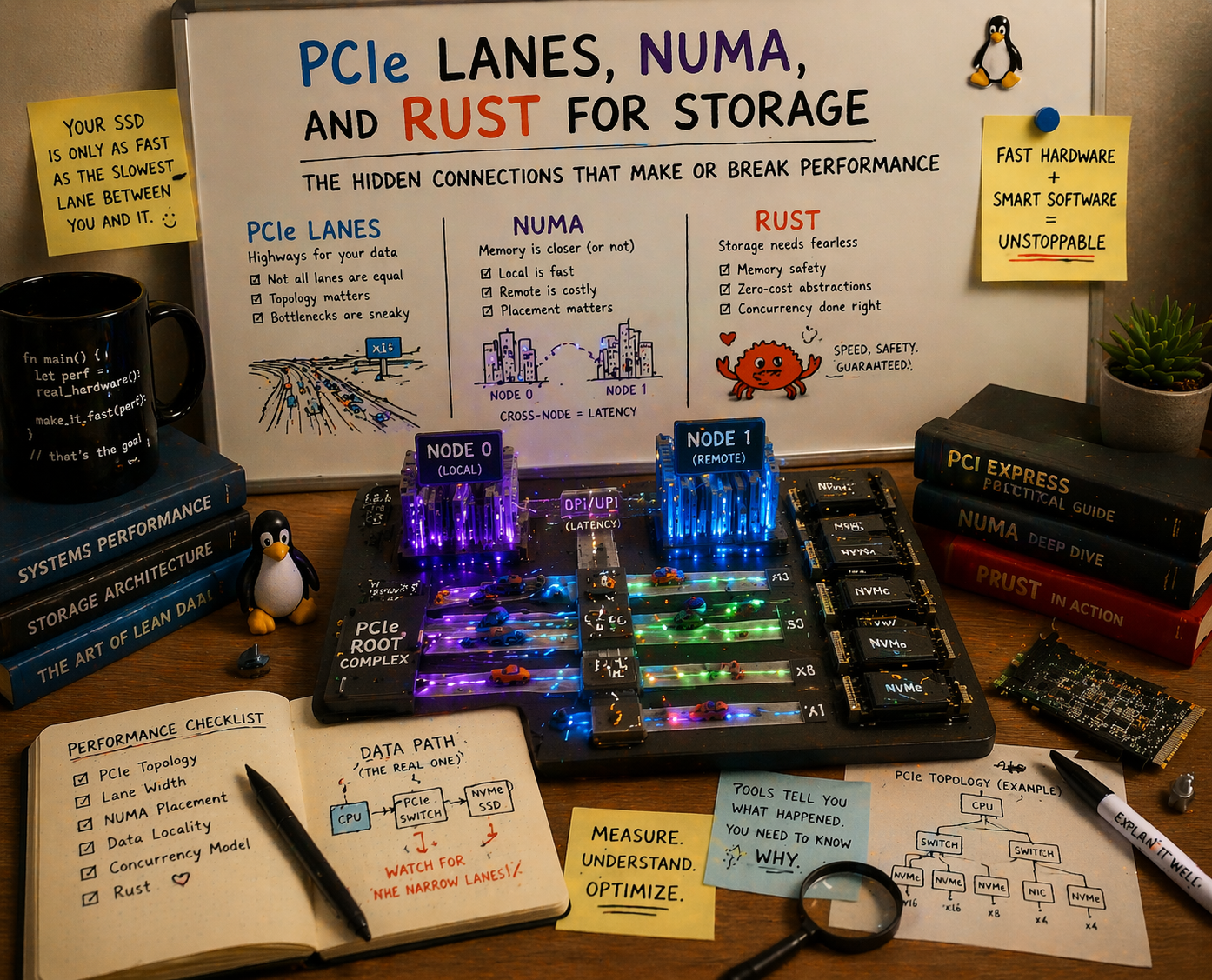
As NVMe counts per chassis climb past 24, 32, and toward 48 drives, the bottleneck shifts from disk speed to PCIe topology. The solution is dual-socket CPUs with massive lane counts, but only if your storage software can actually exploit them without a NUMA penalty. Here’s why Go can’t, and Rust can.
The Lane Crisis: More NVMe Drives Than Your CPU Can Feed
The economics of flash storage are pushing NVMe density to levels that would have been absurd five years ago. With EDSFF E1.S form factors, a 1U server can pack 24 to 32 NVMe drives. In 2U, that number climbs to 36-48 drives. Enterprise SSDs are shipping at 30 TB and 60 TB capacities, meaning a single 2U chassis can hold over a petabyte of raw flash.
But there’s a physics problem. Each NVMe drive requires a PCIe x4 link, four lanes of dedicated bandwidth. The math is brutal:
| Drive Count | PCIe Lanes (NVMe only) | + 2x 100GbE NIC | + Management | Total Needed |
|---|---|---|---|---|
| 24 drives | 96 | +32 | +4 | 132 |
| 32 drives | 128 | +32 | +4 | 164 |
| 48 drives | 192 | +32 | +4 | 228 |
No single-socket CPU on the market today provides 132+ PCIe lanes. The gap between what NVMe-dense chassis demand and what one CPU socket can supply forces one of two compromises:
- PCIe switches to fan out limited CPU lanes to more devices
- Dual-socket CPUs to double the lane count with a second processor
Both have costs. But one of those costs is invisible and language-dependent, and that’s where this story gets interesting.
Option 1: PCIe Switches, the Hidden Bottleneck
When a server has more NVMe drives than available CPU PCIe lanes, the standard industry solution is a PCIe switch (Broadcom’s PEX series). A switch takes a x16 uplink from the CPU and fans it out to, say, 4x NVMe drives at x4 each. On paper, the total downstream bandwidth matches the uplink. In practice, it doesn’t.
The Latency Tax
Every PCIe switch hop adds approximately 700 nanoseconds of latency to every I/O transaction. For a single 4 KB random read from a modern NVMe SSD (which completes in ~10 microseconds), that’s a 7% latency penalty per hop. Stack two switches (common in dense JBOF configurations) and you’re at 14%, before you’ve done anything in software.
The Bandwidth Bottleneck
A PCIe switch doesn’t create bandwidth; it shares an uplink. Four NVMe SSDs behind a x16 PCIe 5.0 switch share 64 GB/s of uplink bandwidth. Each drive can individually sustain 14 GB/s of sequential reads. If all four drives are active simultaneously:
- Aggregate demand: 4 x 14 = 56 GB/s
- Uplink capacity: 64 GB/s
- Headroom: 14%. Enough for sequential, but under mixed random I/O with metadata overhead, this oversubscription becomes real contention
Research from USENIX NSDI 2024 on routable PCIe fabrics measured up to 30% bandwidth degradation when crossing PCIe switch boundaries under realistic workloads, with host-to-device throughput dropping from theoretical maximums to 8.4 GB/s in some configurations.
The Cost
PCIe switches aren’t free. A Broadcom PEX88096 (96-lane PCIe 4.0 switch) adds $200-400 per chip, consumes 15-25W of power, and occupies board real estate. In a 48-drive chassis, you might need 4-6 switches, adding $1,000-2,000 and 60-150W to the BOM, a meaningful fraction of the server’s total cost and thermal budget.
The takeaway: PCIe switches are a necessary evil when CPUs don’t provide enough lanes, but they introduce latency, bandwidth contention, cost, and power overhead that directly degrades storage performance.
Option 2: Dual-Socket, More Lanes, More Problems
The alternative is to use two CPUs, each with its own PCIe root complex, collectively providing enough lanes for direct-attach NVMe without switches. This is where Intel’s Xeon 6 Granite Rapids architecture becomes compelling.
Intel Xeon 6760P: The Lane Count King
The Intel Xeon 6760P (Granite Rapids) offers:
- 88 PCIe 5.0 lanes per socket
- 4 UPI links at 24 GT/s for inter-socket communication
- 64 P-cores at 2.2 GHz base / 3.8 GHz turbo
- 320 MB cache, 8 DDR5-6400 memory channels
- 330W TDP
In dual-socket configuration: 176 PCIe 5.0 lanes total. That’s enough for 32 NVMe drives at x4 each (128 lanes) plus two 100GbE NICs (32 lanes) plus management (4 lanes), 164 lanes used, 12 spare, all directly attached to CPU root complexes with zero PCIe switches.
For comparison:
| Platform | Lanes/Socket | Dual-Socket Total | Notes |
|---|---|---|---|
| Intel Xeon 6760P | 88 PCIe 5.0 | 176 | 4 UPI @ 24 GT/s |
| AMD EPYC 9654 (Genoa) | 128 PCIe 5.0 | 160* | Infinity Fabric consumes lanes |
| AMD EPYC 9654P (single) | 128 PCIe 5.0 | 128 | No NUMA, all lanes for I/O |
| AMD EPYC 9755 (Turin) | 128 PCIe 5.0 | 160* | Same IF tradeoff |
*AMD EPYC dual-socket allocates a portion of each CPU’s Infinity Fabric links to inter-socket communication, reducing usable PCIe lanes. The net gain from adding a second socket is only 32 lanes (160 - 128 = 32), not a full doubling.
Intel’s architecture is different: UPI links are separate from PCIe lanes. Adding a second Xeon 6760P gives you a full additional 88 PCIe lanes without sacrificing any from the first socket. This makes dual-socket Intel uniquely attractive for NVMe-dense configurations.
The NUMA Problem
But dual-socket introduces NUMA (Non-Uniform Memory Access). In a dual-socket system, each CPU has its own local memory and its own PCIe lanes. When a thread on Socket 0 accesses memory attached to Socket 1, it must traverse the inter-socket link (UPI for Intel, Infinity Fabric for AMD), incurring a penalty:
| Access Type | Typical Latency |
|---|---|
| Local memory (same socket) | ~90 ns |
| Remote memory (cross-socket) | ~120-180 ns |
| Penalty | 30-100% overhead |
For a storage system, this means: if a thread on Socket 0 processes an I/O request for an NVMe drive attached to Socket 1, every memory access involved in that I/O (reading the command buffer, copying data, computing checksums) pays the cross-socket tax. At 100,000+ IOPS per drive, this adds up to milliseconds of aggregate penalty per second per drive.
The solution is conceptually simple: pin I/O threads to the same socket as their drives. Socket 0’s threads handle Socket 0’s NVMe drives; Socket 1’s threads handle Socket 1’s. Memory allocations stay local. PCIe transactions stay local. The inter-socket link carries only coordination traffic, not data.
The question is: can your storage software actually do this?
Go’s NUMA Blindness: A Structural Problem
Go, the language behind several major object storage systems, has a fundamental problem with NUMA. It’s not a bug. It’s a design decision that permeates the runtime.
The Goroutine Scheduler Doesn’t Know About Sockets
Go’s runtime scheduler (the GMP model: Goroutines, M threads, P processors) was designed for throughput on uniform memory architectures. It has no concept of NUMA nodes, sockets, or memory locality.
Key behaviors that destroy NUMA performance:
1. Work stealing crosses socket boundaries freely.
When a P (logical processor) runs out of goroutines to execute, it steals work from other P’s, including P’s on the other NUMA node. A goroutine that was allocated its stack, its buffers, and its mcache on Socket 0 can be stolen and resume execution on Socket 1. Every subsequent memory access hits remote DRAM.
The NUMA-aware scheduler proposal by Dmitry Vyukov (2014) acknowledged this problem and designed a solution with per-node run queues and node-local work stealing preferences. It was never implemented. Over a decade later, Go’s scheduler remains NUMA-unaware.
2. Memory allocation is NUMA-oblivious.
Go’s memory allocator (based on TCMalloc) uses per-P mcaches backed by a global mheap. When a goroutine allocates memory, it comes from the OS page that happens to be available, which may be on either NUMA node. There is no mechanism to request node-local allocation, and no per-node memory pools.
The allocator is designed to be fast (lock-free per-P fast path), not local. In a dual-socket system:
- A goroutine on Socket 0 may allocate a 64 KB I/O buffer from Socket 1’s memory
- Every byte copied to/from that buffer pays the cross-socket penalty
- The GC (which scans heap objects) also traverses remote memory, adding to cross-socket traffic
3. The GC generates cross-socket traffic.
Go’s concurrent garbage collector uses multiple worker goroutines that scan the entire heap. GC workers on Socket 0 will scan objects physically located in Socket 1’s DRAM, generating sustained cross-socket memory traffic during every GC cycle. For a storage system under load, which allocates and frees millions of I/O buffers per second, GC cycles are frequent and cross-socket traffic is substantial.
4. runtime.LockOSThread() is a blunt hammer.
Go provides LockOSThread() to pin a goroutine to its current OS thread, and you can then use syscall to set CPU affinity on that thread. But this defeats Go’s scheduler entirely for that goroutine; it can’t be preempted, work-stolen, or multiplexed. Doing this at scale (pinning thousands of I/O-handling goroutines) turns Go’s concurrency model into an expensive wrapper around manual thread management.
The Result: Single-Socket AMD Became the Default
The practical consequence of Go’s NUMA blindness is that the Go storage ecosystem avoided dual-socket systems entirely. AMD’s EPYC P-series (single-socket SKUs) became the de facto choice:
- EPYC 9654P: 96 cores, 128 PCIe 5.0 lanes, single socket, no NUMA
- EPYC 9755P (Turin): 128 cores, 128 PCIe 5.0 lanes, single socket, no NUMA
With 128 lanes, you can direct-attach 24 NVMe drives (96 lanes) with room for networking (32 lanes). No NUMA means Go’s scheduler works fine; all memory is local, all PCIe transactions are local, work stealing has no penalty.
But 128 lanes is the ceiling. For 32+ drive configurations, you either add PCIe switches (with their latency and bandwidth penalties) or you leave performance on the table. Go’s language runtime limits your hardware architecture to single-socket, which in turn limits your NVMe density to what one socket can feed.
This is the invisible tax. No benchmark captures it because nobody benchmarks the configuration they can’t run. The comparison isn’t “Go on dual-socket vs. Go on single-socket” (where dual-socket would lose due to NUMA penalties). The comparison is “Go on single-socket with 24 NVMe drives” vs. “a NUMA-aware system on dual-socket with 48 NVMe drives.” The latter configuration simply doesn’t exist in the Go storage world.
Rust Eliminates the NUMA Tax
Rust gives you the tools to exploit dual-socket systems without paying the NUMA penalty. Not as an afterthought or a workaround, but as first-class capabilities that compose with the language’s ownership and concurrency model.
Thread-to-Core Pinning
Rust’s core_affinity crate and direct libc::sched_setaffinity calls let you pin threads to specific cores with zero overhead:
use core_affinity::CoreId;

// Pin current thread to core 0 (Socket 0)
core_affinity::set_for_current(CoreId { id: 0 });
With tokio, you configure this at runtime initialization:
tokio::runtime::Builder::new_multi_thread()
    .worker_threads(16)
    .on_thread_start(|| {
        // Pin each worker thread to cores on the local NUMA node
        let core_id = determine_local_core();
        core_affinity::set_for_current(core_id);
    })
    .build()
You can run two separate tokio runtimes, one pinned to Socket 0’s cores, one pinned to Socket 1’s cores, each handling I/O for its local NVMe drives. No cross-socket migration, no remote memory access, no NUMA penalty.
NUMA-Aware Memory Allocation
Rust’s custom allocator support (via the Allocator trait and #[global_allocator]) lets you use NUMA-aware allocators like jemalloc with per-NUMA-node arenas, or wrap libnuma’s numa_alloc_onnode() directly:
// Allocate a buffer on NUMA node 0
let buf = numa_alloc_onnode(size, 0);
Because Rust has no GC, once you allocate memory on a specific NUMA node, it stays there until you explicitly free it. No background process will scan it from the wrong socket. No compaction will move it. The allocation is deterministic and local for its entire lifetime.
No GC Crossing Socket Boundaries
This is Rust’s most significant NUMA advantage, and it requires zero code. Because there is no garbage collector:
- No GC worker threads scanning remote DRAM
- No stop-the-world pauses generating cross-socket traffic spikes
- No heap compaction moving objects between NUMA nodes
- No allocation pressure causing the runtime to grab memory from the wrong node
Memory is freed when it goes out of scope. Drop runs on the thread that owns the value, the thread you pinned to the local socket. The entire lifecycle is NUMA-local by construction.
The Dual-Socket Rust Architecture
Here’s what a NUMA-aware Rust storage node looks like on a dual Xeon 6760P system:
Socket 0 (88 PCIe lanes)              Socket 1 (88 PCIe lanes)
├─ 16 NVMe drives (64 lanes)          ├─ 16 NVMe drives (64 lanes)
├─ 1x 100GbE NIC (16 lanes)           ├─ 1x 100GbE NIC (16 lanes)
├─ 8 remaining lanes (management)     ├─ 8 remaining lanes (management)
│                                      │
├─ Tokio runtime A (32 cores)         ├─ Tokio runtime B (32 cores)
│  ├─ Pinned to Socket 0 cores        │  ├─ Pinned to Socket 1 cores
│  ├─ NUMA-local memory pool          │  ├─ NUMA-local memory pool
│  ├─ Handles Socket 0 NVMe I/O       │  ├─ Handles Socket 1 NVMe I/O
│  └─ Local S3 request processing      │  └─ Local S3 request processing
│                                      │
└─ 4 DDR5-6400 channels (local)       └─ 4 DDR5-6400 channels (local)
         │                                      │
         └──────── UPI (4 links x 24 GT/s) ─────┘
                   (coordination only, not data)
32 NVMe drives, all direct-attach, zero PCIe switches, zero NUMA penalty. The UPI links handle only cluster coordination traffic (heartbeats, placement queries, metadata RPCs), not bulk data I/O.
Contrast this with what a Go storage system would have to settle for:
Single Socket AMD EPYC 9654P (128 PCIe lanes)
├─ 24 NVMe drives (96 lanes)  ← maximum without switches
├─ 2x 100GbE NIC (32 lanes)
└─ 0 remaining lanes

OR

├─ 32 NVMe drives (128 lanes) ← requires stealing NIC lanes or adding switches
├─ Networking through PCIe switch (added latency + cost)
The Rust system serves 33% more drives at full bandwidth with no switches, while the Go system either caps at 24 drives or adds switches that degrade every I/O operation.
Looking Forward: The Lane Arms Race
Intel’s leaked Nova Lake platform (expected late 2026) introduces the LGA1954 socket with a new 900-series chipset providing up to 48 additional PCIe lanes from the chipset alone. Combined with CPU-direct lanes, dual-socket Nova Lake systems could push past 200 usable PCIe 5.0 lanes, enough for 48+ direct-attach NVMe drives.
AMD’s roadmap continues to prioritize single-socket density (128-160 lanes), but the next generation of CXL-enabled memory tiering will introduce new NUMA-like topologies where memory can be attached via CXL to either socket, further widening the gap between NUMA-aware and NUMA-oblivious software.
The trend is clear: hardware is providing more PCIe lanes, more NUMA nodes, and more complex memory topologies. Software that can’t exploit this hardware leaves performance, and drive density, on the table.
The Bottom Line
The NVMe density problem is a hardware problem that demands a software solution:
- More NVMe drives per chassis require more PCIe lanes than any single socket provides
- PCIe switches fill the gap but add 700ns+ latency and up to 30% bandwidth degradation
- Dual-socket CPUs (especially Intel Xeon 6760P with 176 total PCIe 5.0 lanes) provide enough lanes for 32+ direct-attach drives
- But dual-socket means NUMA, and NUMA requires software that can pin threads, localize memory, and avoid cross-socket traffic
- Go can’t do this. Its scheduler, allocator, and GC are structurally NUMA-unaware, with a decade-old proposal to fix it that was never implemented
- Rust can. Thread pinning, NUMA-local allocation, no GC, and deterministic memory lifecycle make dual-socket zero-penalty
The Go storage ecosystem’s retreat to single-socket AMD wasn’t a preference; it was a concession. A concession that limits NVMe density, forces reliance on PCIe switches, and leaves 33-50% of potential drive slots unusable.
As NVMe capacities grow and drive counts per chassis climb, the storage software that can exploit dual-socket NUMA hardware without penalty will deliver more capacity, more bandwidth, and lower latency per rack unit than any Go-based alternative. Not because of language speed, but because of hardware utilization that Go’s runtime model structurally prevents.
Intel Xeon 6760P specifications from Intel ARK. AMD EPYC lane allocation behavior documented in AMD’s EPYC 9004 architecture overview. PCIe switch latency measurements from Broadcom documentation and USENIX NSDI 2024. NUMA latency figures from Intel VTune documentation. Go NUMA scheduler proposal from Dmitry Vyukov’s design document. Intel Nova Lake platform details from Tom’s Hardware. Rust NUMA thread pinning via core_affinity crate and tokio affinity guide.
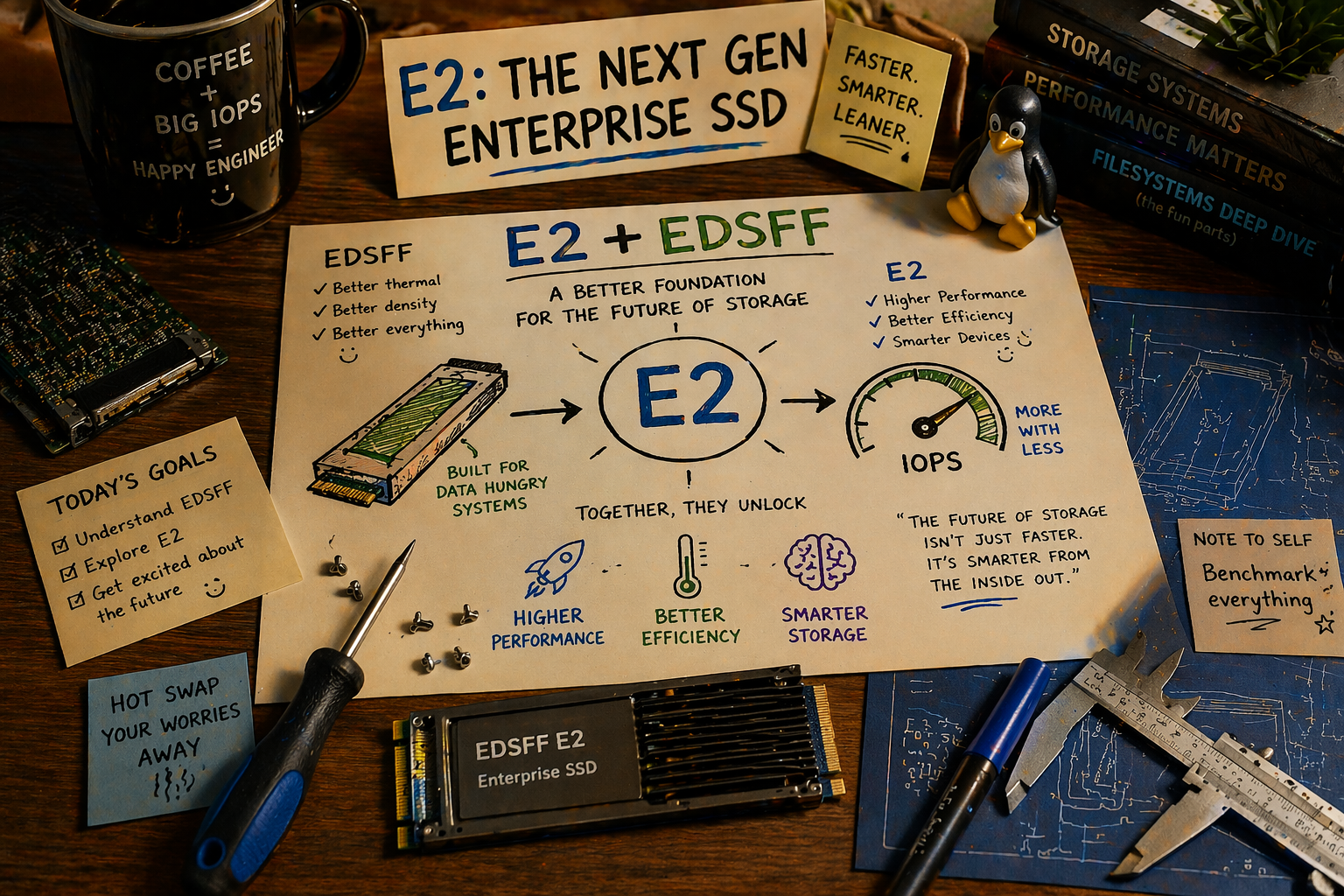
The 2.5-inch drive bay is 26 years old. It was designed for laptop hard drives spinning at 5,400 RPM. Today we’re shoving 122 TB of QLC flash into that same rectangular hole, bolting on a PCIe Gen4 x4 interface, and pretending nothing has changed. Something has changed. EDSFF is the first SSD form factor designed for data centers from scratch, and its newest member, E2, will put a petabyte on a single drive and 40 petabytes in a single 2U server. That’s not just a hardware story. It’s a storage software story, because every assumption your code makes about drive count, failure domains, rebuild times, and power budgets is about to be wrong.
A Brief History of Putting Storage in Boxes
Each form factor transition changed the math for storage software. The transition to EDSFF will be the most consequential since the move from spinning rust to flash.
3.5-Inch HDD (1983-present)
The original. Designed for desktop PCs, adopted by servers because that’s what existed. A 4U chassis holds 36 3.5-inch drives. At 20 TB per HDD (Seagate Exos X20), that’s 720 TB raw in 4U. The form factor assumes mechanical spindles, vibration isolation, and 12V power delivery. Cooling is a non-issue because HDDs generate 5-8W each.
Storage software was designed around this: hundreds of drives per rack, each one slow (200 MB/s sequential), each failure losing 20 TB. Rebuild times of 4-8 hours at full drive speed. RAID-6 or 8+3 erasure coding with enough parity to survive two simultaneous failures during the rebuild window.
2.5-Inch SSD (2007-present)
The laptop form factor that ate the data center. Originally 15mm thick for enterprise (U.2 connector), now the standard NVMe SSD carrier. A 2U chassis holds 24 U.2 SSDs. At 30.72 TB per drive (Samsung PM1733), that’s 737 TB raw in 2U. At Solidigm’s 122.88 TB D5-P5336 (shipping Q1 2025), that’s 2.95 PB raw in 2U. From a 24-bay chassis. Designed for laptop drives.
The 2.5-inch form factor has three problems at these densities:
-
Power delivery. The U.2 connector was designed for 25W. A high-performance NVMe SSD can draw 25-40W under sustained write. Twenty-four drives at 40W is 960W just for storage, in a chassis whose power supply and cooling were designed for 24 drives at 10W each.
-
Airflow. 2.5-inch drives sit perpendicular to the airflow in most chassis designs (drive cages with front-loading trays). Hot air from the front drives heats the rear drives. At 24 drives generating 25W each, thermal throttling in the back row is a real problem.
-
Wasted space. An NVMe SSD doesn’t have a spinning platter. The PCB inside a 2.5-inch SSD uses maybe 60% of the available volume. The rest is air, structural frame, and a connector designed for a different era.
M.2 (2013-present)
The gumstick form factor. Compact, direct-attach via M-key PCIe slot, no cables. Popular in consumer, workstation, and some server boot drives. But M.2 has no hot-swap capability, limited cooling surface area, and maxes out at about 8 TB in the 22110 length. Not a serious data center form factor for bulk storage.
Enter EDSFF: Designed for Data Centers, Not Laptops
EDSFF (Enterprise and Data Center Standard Form Factor) is a family of SSD form factors developed by SNIA’s SFF Technical Work Group, with contributions from Intel, Samsung, Kioxia, Dell, HPE, and 10+ other companies. The specifications define form factors purpose-built for server and storage chassis.
The key insight behind EDSFF: the form factor should serve the flash, not the other way around. Flash packages are flat rectangles. The optimal form factor for packing flash is a flat rectangle. Not a 2.5-inch box designed for a spinning disk, and not a gumstick designed for a laptop motherboard.
The EDSFF Family
| Form Factor | Dimensions (mm) | PCIe Lanes | Max Power | Target Use Case |
|---|---|---|---|---|
| E1.S (short) | 31.5 x 111.49 (5.9mm) | x4 | 12-25W | Boot, caching, mixed-use |
| E1.L (long ruler) | 38.4 x 318.75 (9.5/18mm) | x4 or x8 | 25-40W | Maximum capacity per drive |
| E3.S (short square) | 76.0 x 111.49 (16.8mm) | x4 or x8 | 25-40W | U.2 replacement, performance |
| E3.L (long) | 76.0 x 142.2+ | x4 or x8 | 25-70W | Extreme capacity, AI |
All EDSFF form factors share the SFF-TA-1002 edge connector: a card-edge PCIe interface that eliminates the U.2/SAS cable. No cables means no cable routing, no cable failures, and no airflow obstruction. The drive slides into a backplane slot, makes contact, and starts serving I/O.
E1.S: The Quiet Revolution Already Happening
E1.S is the most widely adopted EDSFF variant today, and it’s eating U.2 from the bottom up. It’s the form factor behind Meta’s, Microsoft’s, and Google’s latest server designs (aligned with the Open Compute Project specifications).
Why E1.S is winning:
- Hot-swappable with a simple latch mechanism (no screw-down like M.2, no tray like U.2)
- Slim enough for 1U. At 5.9mm thick (or 9.5mm/15mm/25mm in taller variants), you can pack 32 E1.S drives vertically in a 1U chassis
- Right-sized power. 12W for a read-heavy caching SSD, 25W for a write-intensive workload. The connector supports up to 70W for future Gen6 drives
- Available now from Samsung, Kioxia, Solidigm, Micron, SK hynix, and Western Digital. Capacities up to 30.72 TB (Kioxia CD8P, Samsung PM9D3a)
Market projections show E1.S growing from 7.2% of total PCIe exabytes shipped in 2022 to 25.9% in 2027, and from 8% of PCIe units to 40.4% of units. The transition is underway.
E1.L: The Ruler That Packs a Petabyte
E1.L is the “ruler” form factor: 318.75mm long (12.5 inches), designed to slide vertically into a 1U chassis from the front. At 38.4mm wide, you can fit 32 E1.L drives in a single 1U row. Intel originally championed this form factor for their 3D XPoint (Optane) ruler drives, but it’s now the natural home for high-capacity QLC flash.
Solidigm’s D5-P5336 is shipping in E1.L form factor at 30.72 TB and 61.44 TB, with the 122.88 TB version sampling. Kioxia’s LC9 Series targets the same form factor at up to 245.76 TB per drive.
The density math with E1.L:
32 x E1.L drives in 1U:

At 61.44 TB/drive:   1.97 PB raw in 1U
At 122.88 TB/drive:  3.93 PB raw in 1U
At 245.76 TB/drive:  7.86 PB raw in 1U
Compare with today’s standard: 24 x U.2 in 2U = 737 TB at 30.72 TB/drive. The E1.L configuration delivers 5-10x the density per rack unit.
E3.S and E3.L: The Performance Tier
E3.S is positioned as the direct U.2 replacement for performance-oriented workloads. It’s wider than E1.S (76mm vs 31.5mm), which gives more PCB area for DRAM cache, power delivery circuitry, and heat spreader contact. E3.S supports x4 or x8 PCIe lanes, enabling higher bandwidth per drive.
Samsung’s PM1743 (TLC) ships in E3.S at up to 15.36 TB. Their BM1743 (QLC) has been demonstrated at FMS 2024 in E3.S, 2.5”, E1.S, and E1.L form factors, with the flagship 122.88 TB model.
E3.L is the newest and most extreme variant. Kioxia’s LC9 Series (announced July 2025) puts 245.76 TB in an E3.L form factor using 32-die stacked BiCS QLC flash with CBA (CMOS Bonded to Array) technology. PCIe 5.0 x4, dual-port capable. 12 GB/s sequential read, 3 GB/s sequential write, 1.3M read IOPS. This is the world’s first quarter-petabyte SSD, and it won “Best of Show” at FMS 2025.
E2: The Petabyte Drive
E1.S, E1.L, E3.S, and E3.L are evolutionary. They’re better shapes for flash packages, optimized for existing server platforms. E2 is something else entirely. It’s a new form factor co-developed by SNIA and OCP specifically to kill the hard drive in warm storage tiers, and the numbers are staggering.
The Spec: SFF-TA-1042
The E2 specification (SFF-TA-1042) was published on June 16, 2025. It defines a ruler-shaped drive with these dimensions:
| Property | E2 Specification |
|---|---|
| Length | 200 mm (7.9 inches) |
| Height | 76 mm (3.0 inches) |
| Thickness | 9.5 mm |
| Interface | PCIe 6.0 x4 (256 GT/s) |
| Connector | SFF-TA-1002 edge + SFF-TA-1009 pinout |
| Max Power | 79.2W (6.6A at 12V) |
| Typical Power | 20-30W (read-heavy workloads) |
| NAND Packages | 64+ minimum |
| Target Capacity | Up to 1 PB per drive |
| Target Throughput | 8-10 MB/s per TB (~10 GB/s at 1 PB) |
| Chassis Fit | 40 drives vertical in 2U |
Read that last line again. Forty E2 drives in a standard 2U rack-mount server. At the target capacity of 1 PB per drive, that’s 40 PB raw in a 2U chassis. A single server. Two rack units.
For context: 40 PB is roughly the total storage capacity of a medium-sized cloud provider’s region. In 2020, that took a data center wing. With E2, it takes a shelf.
How E2 Differs from E1.L and E3.L
E2 is not just a bigger ruler. It’s designed from scratch to achieve a different goal: HDD cost per TB at SSD performance.
| Property | E1.L | E3.L | E2 |
|---|---|---|---|
| Length | 318.75 mm | 142.2+ mm | 200 mm |
| Height | 38.4 mm | 76 mm | 76 mm |
| Target capacity | 61-245 TB | 245 TB | Up to 1 PB |
| NAND packages | 16-32 | 32-64 | 64+ |
| Interface | PCIe 5.0 x4/x8 | PCIe 5.0 x4/x8 | PCIe 6.0 x4 |
| Chassis density | 32 in 1U | 8-16 in 2U | 40 in 2U |
| Performance model | Balanced | Read-heavy | Capacity-optimized |
E2’s design goal is explicit: support at least 64 NAND packages in a single drive, double capacity outside of the NAND technology cadence. Where E1.L and E3.L get bigger by waiting for denser NAND (more layers, more bits per cell), E2 gets bigger by fitting more packages on the PCB. It’s a packaging innovation as much as a silicon innovation.
Who’s Building E2
The E2 specification was presented at the OCP Storage Tech Talk on May 14, 2025, in a panel featuring:
- Micron (demonstrated a 500+ TB prototype)
- Pure Storage (exhibited a 300 TB E2 prototype with large flash controller, six DRAM cache chips, and capacitors for power-loss data protection)
- Meta (shared 3D CAD renders of an E2 server system, defining the chassis and cooling requirements)
- Microsoft (provided requirements from Azure’s warm storage tier)
This isn’t vaporware from a startup. These are the companies that build the world’s largest storage deployments telling SNIA what they need next. When Meta designs a 2U chassis around E2, that chassis will ship in volumes measured in hundreds of thousands.
The Warm Data Target
E2 has a specific workload in mind: warm data. Not the hot tier (frequently accessed, latency-sensitive, served by TLC NVMe). Not the cold tier (rarely accessed, archived, served by HDDs or tape). The warm tier is data accessed occasionally but not constantly: older social media posts, completed ML training datasets, regulatory archives that must be queryable, surveillance footage past the 30-day active window.
Today, warm data lives on HDDs because the cost per TB of QLC SSDs is still 3-5x higher than HDDs. E2’s thesis is that the density advantage (40 PB in 2U vs. 40 PB in multiple racks of HDDs), the performance advantage (10 GB/s vs. 200 MB/s), and the power advantage (20-30W per drive vs. 8-10W per HDD, but serving 50x more TB per watt) will close the TCO gap.
The math: a 4U JBOD chassis holds 60 3.5-inch HDDs at 20 TB each = 1.2 PB raw. A 2U E2 chassis holds 40 drives at 1 PB each = 40 PB raw. To match the E2 chassis capacity with HDDs, you need 33 JBOD chassis (132U, more than three full racks). The floor space, power, cooling, cabling, and operational overhead of 33 chassis vs. 1 is where E2 wins the TCO argument, even if the per-TB media cost is higher.
The 40 PB Server
Let me sketch what a fully populated E2 server looks like:
┌────────────────────────────────────────────────────────────────┐
│  2U E2 Chassis: 40x E2 Drives + Dual-Socket Compute           │
├────────────────────────────────────────────────────────────────┤
│                                                                │
│  Front (drive bays):                                           │
│  ┌──┬──┬──┬──┬──┬──┬──┬──┬──┬──┬──┬──┬──┬──┬──┬──┬──┬──┬──┬──┐
│  │E2│E2│E2│E2│E2│E2│E2│E2│E2│E2│E2│E2│E2│E2│E2│E2│E2│E2│E2│E2│
│  │E2│E2│E2│E2│E2│E2│E2│E2│E2│E2│E2│E2│E2│E2│E2│E2│E2│E2│E2│E2│
│  └──┴──┴──┴──┴──┴──┴──┴──┴──┴──┴──┴──┴──┴──┴──┴──┴──┴──┴──┴──┘
│  40 x E2 @ 9.5mm thick, 76mm tall, vertical in 2U             │
│                                                                │
│  At 500 TB/drive:  20 PB raw     │  At 1 PB/drive:  40 PB raw │
│  After 8+4 EC:     13.3 PB usable│  After 8+4 EC:   26.7 PB   │
│                                                                │
│  Compute: 2x next-gen Xeon or EPYC (PCIe 6.0)                 │
│  Network: 2x 400GbE (or 1x 800GbE)                            │
│  PCIe lanes needed: 40x4 + NIC + mgmt = ~176 lanes            │
│  Power: 40 x 25W avg + CPUs + NIC = ~1,800-2,200W             │
│  Cooling: front-to-back airflow, ruler drives act as chimneys  │
└────────────────────────────────────────────────────────────────┘
A single 42U rack with 21 of these 2U servers: 21 x 20 PB = 420 PB raw (at 500 TB/drive, the near-term target). At 1 PB/drive: 840 PB raw per rack. After erasure coding: roughly 280-560 PB usable per rack.
We’re talking about half an exabyte in a single standard rack. This is a fundamentally different scale than anything storage software has been designed for.
The Software Implications Nobody Is Designing For
Hardware engineers are shipping 245 TB drives in 2025 and prototyping 500 TB+ E2 drives. Storage software engineers are still designing for 8-16 TB drives. This gap will cause real problems.
Problem 1: Rebuild Times
This is the most urgent issue. As I covered in the rebuild time crisis post, reconstruction speed is limited by surviving drive throughput, EC computation speed, and write throughput to replacement drives.
At realistic rebuild rates (500 MB/s sustained, accounting for competing production I/O):
| Drive Capacity | Rebuild Time | Vulnerability Window |
|---|---|---|
| 8 TB | 4.4 hours | Low risk |
| 30 TB | 16.7 hours | Moderate risk |
| 61 TB | 33.9 hours | High risk |
| 122 TB | 67.8 hours (2.8 days) | Very high risk |
| 245 TB | 136 hours (5.7 days) | Unacceptable |
| 500 TB (E2 near-term) | 278 hours (11.6 days) | Catastrophic |
| 1 PB (E2 target) | 555 hours (23.1 days) | Beyond current models |
What software must do:
- Declustered erasure coding. Don’t bind erasure groups to fixed drive sets. Spread parity across all drives so that rebuilding one drive reads from all remaining drives in parallel.
- Prioritized rebuild. Hot data first, cold data later. Rebuild the objects that users are actually reading before rebuilding archival data nobody’s touched in months.
- Partial rebuild. A 245 TB drive may be only 60% full. Only rebuild the objects that actually existed, not the empty space. This cuts rebuild time by 40%.
- Background throttling. Rebuild I/O competes with production I/O. Adaptive throttling that backs off during peak hours and accelerates during off-hours.
Problem 2: Failure Domain Explosion
A 1U chassis with 32 E1.L drives at 122 TB each contains 3.9 PB of raw data. If the chassis fails (power supply, backplane, network switch), you lose 3.9 PB simultaneously. Even with erasure coding protecting against individual drive failures, a chassis-level failure requires a different strategy.
What software must do:
- Cross-chassis erasure coding. The erasure group must span multiple chassis, so that losing one chassis loses at most M shards from any group. This requires network bandwidth for parity distribution but eliminates the chassis as a single failure domain.
- Rack-aware placement. Place shards on different racks when possible, so that a top-of-rack switch failure doesn’t take out an entire erasure group.
- Power domain awareness. In data centers with redundant power feeds, ensure that an erasure group’s shards span both power domains.
This is where deterministic placement algorithms like HRW with failure-domain constraints become essential. The placement function needs to understand the physical topology (drive, chassis, rack, power domain, data center) and ensure that erasure groups span the boundaries that matter.
Problem 3: PCIe Lane Budget
32 E1.L drives at PCIe x4 each = 128 lanes. Add two 100GbE NICs (32 lanes) and you need 160+ lanes. This pushes you into dual-socket territory on Intel (176 lanes with two Xeon 6760P) or requires PCIe switches on AMD single-socket (128 lanes max).
With PCIe Gen5 drives (like the Kioxia LC9 at Gen5 x4), each drive can sustain 14 GB/s reads. Thirty-two drives reading simultaneously is 448 GB/s. This is more than the aggregate memory bandwidth of most dual-socket systems (~400 GB/s for DDR5-6400 x 16 channels). The storage subsystem is now faster than the memory subsystem. Software that buffers I/O through DRAM becomes the bottleneck. Direct I/O (O_DIRECT) and zero-copy I/O paths (io_uring with fixed buffers) become mandatory.
Problem 4: Power and Thermal
32 E1.L drives at 25W each = 800W for storage alone. A 1U chassis with dual-socket CPUs (2 x 350W TDP), networking (50W), and fans (50W) totals 1,550W. That’s approaching the limit of a single 2,000W power supply, and well above the per-rack-unit power budget of most data center designs (which assume 8-12 kW per rack with 42U).
What software must do:
- Power-aware scheduling. Don’t issue concurrent writes to all 32 drives simultaneously. Stagger write operations across drives to stay within the power envelope. Sequential writes are more power-hungry than reads (QLC programming requires higher voltages).
- Thermal monitoring. Read SMART temperature data and throttle I/O to drives approaching thermal limits. NVMe thermal management (TSEL, TMT1/TMT2 thresholds) is exposed via the NVMe admin command set. Storage software should use it.
- Idle power management. Put unused drives into lower power states (NVMe PS1-PS4). A drive in PS3 consumes ~2W instead of 25W. For a chassis with bursty workloads, aggressive power management can cut average storage power by 50%.
Problem 5: QLC Write Endurance
This is the quiet assumption behind every high-capacity EDSFF drive: they’re QLC. Four bits per cell. About 1,000 program/erase cycles before the NAND wears out, compared to 3,000 for TLC and 10,000 for MLC.
The endurance is expressed as DWPD (Drive Writes Per Day over the warranty period). Typical QLC enterprise SSDs are rated at 0.3-1 DWPD for 5 years. At 0.3 DWPD, a 122 TB drive can sustain 36.8 TB of writes per day. That sounds like a lot until you consider:
- Write amplification from erasure coding: 1.5x for 8+4 (writing parity shards)
- Write amplification from the FTL’s internal GC: 2-3x on QLC
- Write amplification from compaction (if you run an LSM-based metadata engine): 10-30x
The aggregate WAF can easily reach 5-10x, meaning 36.8 TB of “allowed” daily writes translates to 3.7-7.4 TB of effective application writes. For a write-heavy workload on a 122 TB drive, that’s a 1.7-3.3% daily utilization ceiling before you’re eating into warranty life.
Samsung’s BM1743 has an additional caveat: a 1-month data retention spec without power. This means the drive is designed for environments where it’s always powered on and data is continuously refreshed. Not a cold storage tier. Not an archival drive. An always-on, read-heavy data lake.
What software must do:
- Write tiering. Use a small TLC/SLC tier (or SLC cache on the QLC drive itself) for write-hot data. Flush to QLC in large, sequential batches. Minimize random writes to QLC.
- Wear monitoring. Track NVMe SMART attributes for percentage used, available spare, and media/data integrity errors. Proactively migrate data off drives approaching end of life.
- Workload-appropriate placement. Write-heavy objects (frequently updated, small, random I/O) should land on TLC drives. Read-heavy, large, sequential objects (Parquet files, video archives, ML training data) belong on QLC.
What’s Actually Shipping (Early 2026)
Let me anchor this in reality. Here are the highest-capacity EDSFF drives available or sampling today:
| Vendor | Model | Capacity | Form Factor | Interface | NAND | Status |
|---|---|---|---|---|---|---|
| Solidigm | D5-P5336 | 122.88 TB | 2.5” U.2, E1.L | PCIe 4.0 x4 | QLC (3D5) | Shipping Q1 2025 |
| Solidigm | D5-P5336 | 61.44 TB | E1.L | PCIe 4.0 x4 | QLC (3D5) | Shipping now |
| Samsung | BM1743 | 122.88 TB | 2.5” U.2, E3.S, E1.S, E1.L | PCIe 5.0 | QLC (V8) | Sampling/demo |
| Kioxia | LC9 Series | 245.76 TB | 2.5”, E3.L | PCIe 5.0 x4 | QLC (BiCS, 32-die stack) | Sampling H2 2025 |
| Samsung | PM1743 | 15.36 TB | E3.S | PCIe 5.0 x4 | TLC (V6) | Shipping |
| Micron | 6550 ION | 61.44 TB | E3.S | PCIe 5.0 x4 | QLC (G8, 232-layer) | Shipping |
| Micron | 6550 ION | 122.88 TB | E3.L | PCIe 5.0 x4 | QLC (G8, 232-layer) | Sampling |
| Kioxia | CD8P | 30.72 TB | E1.S, E3.S | PCIe 5.0 x4 | TLC (BiCS) | Shipping |
The trajectory is clear: 30 TB today, 60 TB common, 122 TB shipping, 245 TB sampling. Micron’s 6550 ION adds another player at the 60-120 TB tier with competitive sequential read (12 GB/s) and the density advantages of their 232-layer G8 NAND. By 2027, 500 TB per drive is plausible with PLC (5 bits/cell) and continued die-stacking improvements.
The 1 PB Node: An Architecture Sketch
What does a storage node look like when a single 1U chassis holds a petabyte?
┌─────────────────────────────────────────────────────────┐
│  1U EDSFF Chassis: 32x E1.L + Dual-Socket Xeon 6760P   │
├─────────────────────────────────────────────────────────┤
│                                                         │
│  Socket 0 (88 PCIe 5.0 lanes)                          │
│  ├── 16x E1.L NVMe @ 30.72 TB each = 491 TB (64 lanes)│
│  ├── 1x 200GbE NIC (16 lanes)                          │
│  ├── Management + boot (8 lanes)                        │
│  ├── 4x DDR5-6400 channels (256 GB)                    │
│  └── Async runtime A (32 cores, pinned)                │
│                                                         │
│  Socket 1 (88 PCIe 5.0 lanes)                          │
│  ├── 16x E1.L NVMe @ 30.72 TB each = 491 TB (64 lanes)│
│  ├── 1x 200GbE NIC (16 lanes)                          │
│  ├── Management + boot (8 lanes)                        │
│  ├── 4x DDR5-6400 channels (256 GB)                    │
│  └── Async runtime B (32 cores, pinned)                │
│                                                         │
│  Total: 983 TB raw                                      │
│  After 8+4 EC: 655 TB usable                           │
│  Power: ~1,400W (32 drives x 25W + 2 CPUs + network)   │
│  Network: 2x 200GbE = 400 Gbps = 50 GB/s aggregate     │
└─────────────────────────────────────────────────────────┘
With Solidigm 61.44 TB E1.L drives, the same chassis holds 1.97 PB raw. With the 122.88 TB version: 3.93 PB raw.
A 42U rack of these nodes: 42 x 983 TB = 40.3 PB raw per rack. After 8+4 erasure coding: 26.9 PB usable per rack. In a standard data center cabinet, on standard power.
For context: a traditional Ceph cluster achieving 26 PB usable might use 6-8 racks of 4U servers with 3.5-inch HDDs. The EDSFF configuration achieves the same capacity in a single rack, with flash-speed performance.
The Software Stack for This Node
The storage software running on this node needs capabilities that most current systems lack:
-
NUMA-aware I/O pinning. Two separate async runtimes, each pinned to its socket’s cores, handling I/O only for locally-attached drives. Cross-socket traffic limited to coordination, not data.
-
32-drive interrupt steering. Each NVMe drive generates interrupts via MSI-X. With 32 drives, the system needs interrupt affinity configuration that distributes interrupt handling across cores on the correct NUMA node. Default Linux behavior (irqbalance) doesn’t understand this.
-
io_uring with registered buffers. At 32 drives x 14 GB/s each = 448 GB/s of potential read throughput, the system is I/O-bound, not CPU-bound. io_uring’s registered buffer and fixed-file modes eliminate per-I/O syscall overhead. Traditional read/write syscalls can’t keep up.
-
Cross-chassis erasure coding. Shards from a single object must span at least 3 chassis to survive a chassis failure. This means 12 RPC calls per PUT (for 8+4 EC), each writing a shard to a different chassis over the 200GbE fabric.
-
Wear-aware shard placement. Don’t write new objects to drives that are already at 80% wear life. Redirect writes to younger drives. This requires reading SMART data periodically and incorporating drive health into the placement algorithm.
The Data Center Impact
The ripple effects of 1 PB/1U extend beyond the storage node:
Network
If each 1U node has 50 GB/s of network bandwidth and 450 GB/s of storage bandwidth, the network is the bottleneck by a factor of 9x. This means:
- Most data stays local. Object storage workloads that can be served from local drives (single-node reads) use 0% of the network. Only cross-node operations (erasure coding writes, healing, rebalancing) consume network bandwidth.
- 400GbE becomes mandatory. Two 200GbE NICs (or one 400GbE NIC) per 1U node. The uplink to the spine switch must be 400GbE or 800GbE. Network infrastructure cost per rack increases significantly.
- Compression pays more. Every byte saved by compression is a byte that doesn’t traverse the network. LZ4 compression at 2:1 ratio effectively doubles your network bandwidth for EC writes.
Power
At 1,400W per 1U node, a 42U rack draws ~59 kW. Most data centers are designed for 8-15 kW per rack. High-density deployments exist (30-50 kW/rack for GPU clusters), but they require liquid cooling or rear-door heat exchangers. EDSFF storage racks may need the same cooling infrastructure previously reserved for AI compute.
Operational Model
When a single 1U chassis holds a petabyte, operational procedures change:
- Drive replacement is a 30-second hot-swap (latch, pull, insert), but the rebuild takes days. Operations teams need monitoring dashboards that track rebuild progress per drive and alert when rebuild time exceeds the safe window.
- Chassis failure is a multi-petabyte event. Runbooks need procedures for “chassis offline, 4 PB at risk.” If erasure coding spans chassis (as it should), the data is safe, but the degraded state affects multiple erasure groups simultaneously.
- Firmware updates are higher-stakes. Updating NVMe firmware on a 245 TB drive while it’s serving production traffic requires careful sequencing. A firmware bug that causes a drive to go offline during the update takes 245 TB out of the cluster for the duration of the rebuild.
Conclusion
The EDSFF family tells a story in three acts. Act one is already playing out: E1.S is replacing U.2 in hyperscale deployments, quietly and without drama. Act two is starting now: E1.L and E3.L drives at 122-245 TB are forcing storage software to rethink rebuild times, failure domains, and power budgets in ways that most production systems aren’t ready for.
Act three is E2. A petabyte per drive. Forty drives in a 2U chassis. Forty petabytes behind a single backplane. When Micron demos a 500 TB prototype and Meta designs the chassis around it, this isn’t a research project. It’s a roadmap item.
E2 breaks assumptions that E1.L merely stresses. A 23-day rebuild time for a 1 PB drive isn’t a scaling problem you solve with faster hardware. It’s a fundamental redesign of how storage software thinks about durability. Traditional rebuild (read everything, recompute parity, write everything back) doesn’t work when “everything” is a petabyte. You need incremental, object-granular healing. You need erasure groups that span chassis so that a single drive failure never puts more than a fraction of its data at risk. You need placement algorithms that understand not just racks and power domains but the economic reality that the drive you lost costs more than some cars.
The form factor is changing. The software needs to change faster.
EDSFF specifications: SFF-TA-1006 (E1.S), SFF-TA-1007 (E1.L), SFF-TA-1008 (E3.S), SFF-TA-1002 (connector), SFF-TA-1042 (E2), maintained by SNIA SFF Technical Work Group. Micron E2 500 TB prototype and warm storage thesis from Micron blog. Pure Storage 300 TB E2 prototype from StorageReview. Solidigm D5-P5336 122.88 TB from ServeTheHome. Samsung BM1743 128 TB from AnandTech at FMS 2024. Kioxia LC9 245.76 TB from Kioxia press release and Tom’s Hardware. EDSFF market share projections from Kioxia/Meta E1.S white paper. Intel Xeon 6760P PCIe lane counts from Intel ARK. Samsung PM1743 E3.S from Samsung Semiconductor. QLC endurance characteristics from SNIA SSSI.

Drive capacities are growing exponentially. Rebuild speeds aren’t. A 20TB HDD rebuild takes 2-5 days. A 60TB HDD rebuild takes 6-9 days. A 122TB QLC SSD, already shipping, takes 5-14 hours even on NVMe Gen4. During every hour of that rebuild window, a second drive failure means data loss. The storage industry’s dirty secret: RAID and traditional erasure coding were designed for drives that rebuild in minutes, not days. We’re still using those designs. The drives moved on.
The Math That Kills
There are two trend lines in storage, and they’re diverging catastrophically.
Drive capacity is exponential. HDD capacity doubles roughly every 3-4 years: 1TB in 2007, 10TB in 2015, 20TB in 2020, 30TB in 2024, 36TB in 2025. Seagate’s HAMR roadmap targets 50TB by 2028 and 100TB by 2030. SSDs are worse: QLC NAND is pushing past HDDs in raw capacity. Solidigm shipped a 122TB QLC SSD (D5-P5336) in Q1 2025. They’ve confirmed 245TB for late 2026. Samsung showed a 128TB-class BM1743 at FMS 2024. The 200TB+ SSD is not a question of if, but when.
Rebuild speed is linear. HDD sequential throughput has been flat at 200-250 MB/s for over a decade. A 2015 HDD and a 2025 HDD read at roughly the same rate; the platters spin at 7200 RPM regardless of capacity. NVMe SSDs are faster (7 GB/s for Gen4, 14 GB/s for Gen5), but sustained rebuild throughput is 30-50% of peak because foreground I/O competes for the same drive bandwidth.
The result is a chart shaped like an opening jaw:
Capacity          ▓▓▓▓▓▓▓▓▓▓▓▓▓▓▓▓▓▓▓▓▓▓▓▓▓▓▓▓▓▓▓▓▓▓▓▓▓▓▓ → exponential
                  ▓▓▓▓▓▓▓▓▓▓▓▓▓▓▓▓▓▓▓▓▓▓▓▓▓
                  ▓▓▓▓▓▓▓▓▓▓▓▓▓▓▓▓▓
                  ▓▓▓▓▓▓▓▓▓▓
                  ▓▓▓▓▓▓
                  ▓▓▓▓
Throughput        ░░░░░░░░░░░░░░░░░░░░░░░░░░░░░░░░░░░░░░░ → flat
                  2007    2015    2020    2025    2030
Rebuild time equals capacity divided by throughput. Capacity grows exponentially. Throughput grows linearly (for SSDs) or not at all (for HDDs). The rebuild window, the hours during which your data is running on reduced redundancy, is growing without bound.
The Rebuild Time Table
Let me be precise. These are calculated rebuild times at realistic sustained throughput (30-50% of max drive speed, accounting for competing foreground I/O):
HDD (at 75-125 MB/s sustained rebuild throughput)
| Drive Capacity | Optimistic (125 MB/s) | Pessimistic (75 MB/s) |
|---|---|---|
| 20 TB | 44 hours (1.9 days) | 74 hours (3.1 days) |
| 30 TB | 67 hours (2.8 days) | 111 hours (4.6 days) |
| 36 TB | 80 hours (3.3 days) | 133 hours (5.6 days) |
| 60 TB | 133 hours (5.6 days) | 222 hours (9.3 days) |
| 100 TB | 222 hours (9.3 days) | 370 hours (15.4 days) |
NVMe SSD (at 2.5-5 GB/s sustained rebuild throughput)
| Drive Capacity | NVMe Gen5 (5 GB/s) | NVMe Gen4 (2.5 GB/s) |
|---|---|---|
| 30 TB | 1.7 hours | 3.3 hours |
| 60 TB | 3.3 hours | 6.7 hours |
| 122 TB | 6.8 hours | 13.6 hours |
| 200 TB | 11.1 hours | 22.2 hours |
| 245 TB | 13.6 hours | 27.2 hours |
A 30TB HDD takes nearly 3-5 days to rebuild. 30TB drives are shipping today. They’re mainstream. And 3-5 days of reduced redundancy is a window large enough to drive a truck through.
Even NVMe SSDs, 30-50x faster than HDDs, can’t fully escape the problem at large capacities. A 122TB SSD, already shipping from Solidigm, takes 7-14 hours to rebuild. A 245TB SSD (shipping late 2026) will take 14-27 hours. These aren’t theoretical numbers. This hardware exists.
ZFS operators already feel this pain. TrueNAS community forums report 5+ days to resilver 20TB drives in a RAIDZ2 vdev of 12 drives. One user estimated 10 days, 7 hours for a full resilver. The canonical advice, “never exceed 12 drives per vdev,” is an admission that the rebuild time problem has already broken the RAIDZ model at current capacities.
Why Rebuild Time Is the Dominant Durability Factor
Storage durability is measured in “nines.” 99.999999999% (eleven nines) durability means you lose one object in 100 billion per year. This is S3’s published durability target. The math behind these nines is MTTDL: Mean Time To Data Loss.
For an erasure-coded system with M parity shards, MTTDL follows this relationship:
MTTDL ∝ MTTF^(M+1) / MTTR^MWhere:
- MTTF = Mean Time To Failure per drive (inversely proportional to Annual Failure Rate)
- MTTR = Mean Time To Repair (rebuild time)
- M = number of parity shards (fault tolerance)
The crucial insight is the exponent on MTTR. For double parity (M=2):
Doubling rebuild time quarters your MTTDL.
For triple parity (M=3): doubling rebuild time reduces MTTDL by 8x. For quad parity (M=4): 16x. The relationship is exponential in the parity count. Every increase in rebuild time compounds super-linearly against your durability guarantee.
A Worked Example
Consider a 12-drive erasure group with 8+4 coding (4 parity shards, tolerates 4 simultaneous failures):
- AFR = 1.5% (enterprise HDD, per Backblaze 2025 fleet data: 1.36%)
- MTTF = 584,000 hours
- 20TB HDD, MTTR = 55 hours
MTTDL = MTTF^5 / (C(12,5) * 5! * MTTR^4)
      = enormous / (792 * 120 * 9,150,625)
      ≈ billions of years
Now swap in a 60TB HDD with MTTR = 180 hours:
MTTR ratio: 180/55 = 3.27x
MTTDL impact: 3.27^4 = 114x worse
The same EC scheme, the same drives, the same failure rate, just larger capacity, and durability drops by two orders of magnitude. You didn’t change anything in your design. The drives just got bigger.
This is the rebuild time crisis in a single equation. Drive vendors ship bigger drives. Your rebuild time goes up. Your MTTDL goes down. And you didn’t do anything wrong.
The Double-Failure Window
MTTDL is an average. Let me make it concrete: what’s the probability that a second drive fails during a rebuild?
For a 12-drive EC group at 1.5% AFR, with 11 surviving drives during rebuild:
P(second failure) ≈ (N-1) × T × AFR / 8760| Rebuild Time | P(2nd failure in group) |
|---|---|
| 8 hours (NVMe, 30TB) | 0.015% |
| 55 hours (HDD, 20TB) | 0.104% |
| 111 hours (HDD, 30TB) | 0.210% |
| 222 hours (HDD, 60TB) | 0.419% |
| 370 hours (HDD, 100TB) | 0.697% |
These look small. They’re not.
In a fleet of 10,000 drives organized in 12-drive EC groups, you’ll have roughly 150 drive failures per year (at 1.5% AFR). Each failure opens a rebuild window. The fleet-wide probability of at least one double failure during any rebuild window in a year:
| Fleet Size | Failures/Year | P(double failure, any group, per year), 20TB HDD |
|---|---|---|
| 100 drives | 1.5 | ~0.16% |
| 1,000 drives | 15 | ~1.6% |
| 10,000 drives | 150 | ~14.8% |
| 100,000 drives | 1,500 | ~80%+ |
At 10,000 HDDs, there’s a 15% annual chance of a double failure during a rebuild. At 100,000 HDDs, it’s a near-certainty. And this is with 20TB drives. With 60TB HDDs, double the probabilities. With 100TB HDDs, triple them.
This is with 4 parity shards. With only 2 parity (RAID-6), a double failure is data loss. With 4 parity, a double failure means you’re down to 2 remaining parity, still alive, but one more failure away from loss. A triple failure during a prolonged rebuild of a 60TB HDD is not impossible. It’s a fleet-level probability that actuaries would refuse to ignore.
The URE Multiplier
As if the double-failure window weren’t enough, there’s a compounding factor that most rebuild time analyses ignore: Unrecoverable Read Errors (UREs).
Every drive has a specified URE rate, the probability that a read returns an error instead of data. For enterprise drives:
| Drive Type | URE Rate | One Error Per |
|---|---|---|
| Consumer HDD | 10^14 bits | 12.5 TB |
| Enterprise HDD | 10^15 bits | 125 TB |
| Enterprise SSD | 10^17-10^18 bits | 12.5-125 PB |
During a rebuild, you must read the entire contents of every surviving drive in the EC group. For a 12+4 EC scheme with 30TB drives, rebuilding one drive means reading 15 surviving drives x 30TB = 450TB.
The probability of hitting at least one URE during that 450TB read:
| Drive Type | P(URE during 450TB rebuild read) |
|---|---|
| Consumer HDD | 100% (guaranteed) |
| Enterprise HDD | 36% |
| Enterprise SSD | 0.36% |
A 36% chance of hitting a URE during rebuild of enterprise HDDs. That URE is effectively another drive failure for that specific stripe; you’ve lost another shard’s worth of data for those sectors. With only double parity, one URE during a single-drive rebuild leaves you at single parity for that stripe. If you’re unlucky enough to hit two UREs on different surviving drives during the same rebuild, you lose data.
This is why RAID-5 is dead. With single parity, any URE during rebuild is data loss. At 30TB drive capacities, the probability of a URE during rebuild with consumer HDDs is essentially 100%. Even with enterprise HDDs, it’s 3-4%. IBM published “Re-evaluating RAID-5 and RAID-6” explicitly warning that RAID-5 is unsuitable for drives above ~12TB.
SSDs are dramatically better. Enterprise SSD URE rates are 1,000x lower than enterprise HDDs. This is an underappreciated advantage of NVMe over HDD for erasure-coded storage. The URE risk during rebuild is negligible for SSDs, while it’s a meaningful contributor to data loss probability for HDDs at current capacities.
How the Industry Copes (and Where It Falls Short)
NetApp: Triple Parity (RAID-TEC)
NetApp addressed the rebuild time crisis head-on by making triple parity the default for all HDDs 6TB and larger. RAID-TEC (Triple Erasure Coding) tolerates 3 simultaneous drive failures, with a default group size of 23 drives (20 data + 3 parity). NetApp estimates ~12 hours to rebuild a 15.3TB SSD and ~30 hours for a 30TB HDD.
The logic is sound: if double failures during rebuild are becoming probable, add a third parity so that even a double failure during rebuild doesn’t lose data. But RAID-TEC is a defensive measure, not a solution. At 60TB HDDs, the rebuild window stretches to 5+ days, and the triple-failure probability during that window starts to matter. Quadruple parity is the obvious next step, and indeed, wide EC codes with 4 parity shards are becoming standard.
Ceph: Declustered Recovery via Placement Groups
Ceph’s architecture naturally declusters data across all OSDs in a pool via Placement Groups (PGs) distributed by CRUSH. When an OSD fails, its PGs are spread across many surviving OSDs, so dozens or hundreds of OSDs participate in recovery, both reading source data and writing rebuilt shards.
This is the right idea. If a traditional 12-drive RAID group loses one drive, 11 drives participate in rebuild. If a Ceph pool has 100 OSDs, all 99 participate. The parallelism scales with cluster size, not EC group size.
The problem is Ceph’s defaults. osd_max_backfills = 1 limits each OSD to one concurrent backfill operation. osd_recovery_op_priority = 3 gives recovery very low priority versus client I/O. With default settings, users report 350 MB/s recovery at best. Tuning to osd_max_backfills = 8-16 raises this to 700+ MB/s per OSD, but operators are conservative. Aggressive recovery settings can noticeably impact foreground latency, and the tuning requires understanding the I/O profile of the cluster.
Ceph has the architecture for fast rebuilds but defaults to slow ones, and most operators never change the defaults.
Per-Object Healing in Object Storage
Some object storage systems don’t rebuild drives. They heal objects.
When a drive fails, there’s no volume-level reconstruction. Instead, a background scanner and on-read healing mechanism repair individual objects. Each object is independently erasure-coded, so healing one object means reading its surviving shards from peer drives, reconstructing the missing shard, and writing it to the replacement drive.
The advantages are significant:
Sparse rebuild. Only actual objects are reconstructed. A 30TB drive with 18TB of data only rebuilds 18TB, a 40% reduction versus full-drive rebuild.
On-read prioritization. When a GET request hits an object that has a missing shard, the system immediately reconstructs it, repairs the shard, and serves the request. Hot data is healed first, as a side effect of being accessed.
No dedicated rebuild I/O. Healing is interleaved with normal operations. There’s no “rebuild mode” that changes the system’s behavior. The scanner runs continuously, and heals are queued alongside client I/O.
The disadvantage: this approach is not designed for speed. A typical scanner checks a fraction of objects per pass, cycling through all objects over multiple passes. This is thorough but slow. After a drive failure, full recovery of all objects can take hours to days, depending on the object count and scanner throughput.
VAST Data: Locally Decodable Erasure Codes
VAST Data takes the most radical approach. Their Locally Decodable Erasure Codes (LDEC) use extremely wide stripes, typically 150 data + 4 parity, across an entire DASE (Disaggregated Shared Everything) cluster.
The key innovation: LDEC allows reconstructing a lost strip by reading only 1/4th of surviving data strips, not all K. For a 150+4 scheme, rebuilding one strip reads ~42 strips instead of 150. This is a fundamental property of the code construction, not an optimization on top of Reed-Solomon.
The result: 2.7% storage overhead (150+4), 4 fault tolerance, and rebuild read amplification equivalent to a much narrower code. VAST claims 60 million years MTTDL and throttles rebuild to ~30 hours per SSD, intentionally slow to minimize foreground impact, because the LDEC’s low read amplification makes even throttled rebuilds safe.
This is the most advanced production answer to the rebuild time crisis, but it requires VAST’s full DASE architecture. It’s not a technique you can bolt onto a traditional storage system.
What a Rebuild-Resilient Architecture Looks Like
The rebuild time crisis isn’t solvable by any single technique. It requires a layered approach where each layer reduces the risk that the layers below it can’t handle.
Layer 1: Wide Erasure Codes with 4+ Parity
The first line of defense: tolerate more simultaneous failures. With 4 parity shards, you can lose 4 drives simultaneously before data loss. During a single-drive rebuild, you’re running at 3 parity, still safe against a double failure plus a URE.
| EC Scheme | Fault Tolerance | Storage Overhead | Sweet Spot |
|---|---|---|---|
| 4+2 | 2 | 50% | Small clusters, <12 drives |
| 8+4 | 4 | 50% | Medium clusters, 12-24 drives |
| 12+4 | 4 | 33% | Large clusters, good efficiency |
| 16+4 | 4 | 25% | Very large clusters, high efficiency |
8+4 is the pragmatic minimum for any system deploying drives larger than 20TB. The 50% overhead is the same as 4+2, but you get double the fault tolerance. There is no reason to use 4+2 on hardware where a single drive failure opens a multi-day rebuild window.
Layer 2: Declustered Placement
Don’t lock data into fixed RAID groups. Distribute erasure-coded shards across all drives in the system using consistent hashing (CRUSH, HRW, or similar). When a drive fails, every surviving drive in the cluster participates in the rebuild, reading its share of the lost drive’s data and writing reconstructed shards.
The speedup is proportional to the ratio of pool size to EC group size. If your EC groups are 12 drives but your cluster has 120 drives, rebuild parallelism increases 10x. If you have 1,200 drives, 100x.
Traditional RAID (12-drive group, 1 drive fails):
    11 drives read → 1 hot spare writes
    Bottleneck: single spare drive's write throughput

Declustered (120-drive cluster, 1 drive fails):
    119 drives read (proportionally) → 119 drives write (proportionally)
    Bottleneck: aggregate cluster bandwidth
Layer 3: Sparse Rebuild
Only rebuild data that actually exists. A 60TB drive at 65% utilization has 39TB of data and 21TB of free space. Traditional RAID rebuilds all 60TB. Object storage rebuilds 39TB, a 35% reduction.
This sounds obvious, but it requires the rebuild engine to know which blocks are allocated. Traditional hardware RAID controllers don’t have this information. Filesystem-integrated RAID (ZFS, IBM Spectrum Scale) does. Object storage systems do inherently. You can enumerate the objects on a failed drive and rebuild exactly those objects.
Layer 4: Prioritized Healing
Not all data is equally urgent. An object being actively served to inference workers needs its redundancy restored immediately. A cold archival object that hasn’t been accessed in 6 months can wait.
A priority-based healing queue orders repair by:
-
Criticality. Objects that have lost the most shards (down to minimum quorum) rebuild first. An object at 8+2 surviving shards (lost 2 of 4 parity) is more critical than an object at 8+3 (lost 1).
-
Hotness. Objects with recent access are rebuilt before cold objects. If the healing engine is competing with foreground I/O for bandwidth, healing hot objects reduces the chance that a GET request hits a degraded object.
-
Age. Older unrebuilt shards are prioritized over newer ones, preventing starvation.
Layer 5: Proactive Healing (Background Scrubbing)
The cheapest rebuild is the one that never happens. Background scrubbing, reading every shard, verifying its checksum, and repairing any corruption found, catches problems before they combine with a drive failure.
A shard with a silent checksum mismatch (bit rot, firmware bug, SDC) is one fewer good shard for reconstruction if a drive fails. If a 12-shard object has 1 silently corrupted shard and then loses a drive, it’s effectively down to 10 healthy shards instead of 11. With 4 parity, that’s still recoverable. With 2 parity, it’s not.
Proactive healing eliminates these silent failures before they compound. A background scanner that verifies every shard on a 30-day cycle means no silent corruption persists for more than a month. Combined with on-read verification (check the checksum on every GET), the probability of encountering a silently corrupted shard during a rebuild approaches zero.
Layer 6: Design for 200TB Drives Today
This is the most important principle and the one most teams ignore. Your storage system’s rebuild architecture should be designed for the largest drive you’ll deploy in 5 years, not the largest drive you’re deploying today.
If you’re deploying 30TB NVMe SSDs in 2025, you should be designing your rebuild strategy for 120-200TB SSDs. That means:
- Rebuild time budget: assume 12-24 hours, not 2-4 hours
- EC width: 4 parity minimum, preferably adaptive
- Declustering: mandatory, not optional
- Prioritized healing: a first-class subsystem, not an afterthought
- Monitoring: real-time rebuild progress dashboards, not “check back tomorrow”
If your architecture handles 200TB drives gracefully, it’ll handle 30TB drives trivially. The reverse is not true.
The Read Amplification Problem
There’s a cost to rebuilding that goes beyond time: read amplification. To reconstruct one lost shard using Reed-Solomon erasure coding, you must read K surviving data shards. For wider EC codes, K is larger:
| EC Scheme | Shards Read per Rebuild | Read Amplification |
|---|---|---|
| 4+2 | 4 | 4x |
| 8+4 | 8 | 8x |
| 12+4 | 12 | 12x |
| 16+4 | 16 | 16x |
For a 16+4 scheme with 30TB drives, rebuilding one drive means reading 16 x 30TB = 480TB from surviving drives. At 3 GB/s sustained per NVMe drive, that’s 160 seconds per drive x 16 drives = about 44 minutes of wall-clock time (with parallelism). But the aggregate I/O is 480TB, bandwidth that competes with client requests.
In a distributed system where shards are spread across nodes, this read amplification becomes network traffic. Rebuilding a 30TB drive in a 16+4 scheme transfers 480TB across the network. At 100 Gbps (12.5 GB/s), that’s 10.7 hours of sustained wire-rate transfer. At 25 Gbps per link, it’s 42 hours. Network bandwidth, not drive speed, becomes the bottleneck for cross-node rebuild.
Meta documented this: in their HDFS clusters, erasure-coded recovery generated 180TB per day of cross-rack network traffic just for repair. This consumed meaningful fractions of their TOR switch bandwidth and impacted MapReduce job performance.
Reducing Read Amplification
Three approaches exist:
Locally Decodable Codes (VAST’s LDEC). Algebraically designed so that each lost symbol can be reconstructed by reading a small subset (e.g., 1/4th) of surviving symbols. For 150+4, rebuilding reads ~42 strips instead of 150. This reduces read amplification by 3.5x at the cost of code construction complexity.
Minimum Storage Regenerating (MSR) codes. MSR codes (including Clay codes, published at USENIX FAST 2018) achieve the information-theoretic minimum repair bandwidth. For a (10,4) code, Clay codes reduce repair bandwidth by 2.9x compared to Reed-Solomon, with only 1.25x storage overhead. Ceph has implemented Clay codes as an experimental EC backend.
Multi-Level Erasure Coding (MLEC). Use fast, narrow local EC within each node (e.g., 4+2 across local drives) and wide global EC across nodes (e.g., 8+4 across nodes). Local drive failures are repaired locally, zero network traffic. Only correlated failures (node loss, rack loss) trigger global repair. Research from UChicago (SC’23) showed MLEC reduces repair network traffic by orders of magnitude versus single-level EC.
Each of these is a production-ready technique (LDEC at VAST, Clay codes in Ceph, MLEC in research). The storage systems of 2030, facing 200TB drives, will need all three.
The HDD vs SSD Calculation
Everything I’ve described is worse for HDDs than SSDs. Let me quantify how much worse.
| Factor | HDD (30TB) | NVMe Gen4 SSD (30TB) | SSD Advantage |
|---|---|---|---|
| Rebuild throughput | 75-125 MB/s | 2.5-3.75 GB/s | 20-50x faster |
| Rebuild time | 67-111 hours | 2.2-3.3 hours | 20-50x shorter |
| URE rate | 10^15 (enterprise) | 10^17-10^18 | 100-1,000x better |
| P(URE during rebuild) | 14-36% | 0.04-0.36% | 40-1,000x lower |
| AFR | 1.0-2.0% | 0.5-1.0% | 2x better |
SSDs address the rebuild time crisis at every level: faster rebuild, fewer UREs during rebuild, lower failure rate, shorter vulnerability window. The total durability improvement from switching HDD to NVMe SSD for the same capacity is not 20-50x (the throughput ratio). It’s multiplicative across all factors, easily 1,000x+ improvement in effective MTTDL.
This is why the all-flash datacenter isn’t just about performance. It’s about durability. At 60TB+ drive capacities, HDDs cannot rebuild fast enough to maintain acceptable durability without heroic engineering (LDEC, triple parity, aggressive declustering). SSDs maintain acceptable rebuild windows at current capacities and have headroom for 200TB+.
The remaining argument for HDDs, cost per TB, is narrowing. QLC NAND is closing the gap. A 60TB QLC SSD is cheaper per TB than a 60TB HAMR HDD would be, and it rebuilds 20-50x faster. The TCO calculation must include the durability benefit, not just the acquisition cost.
Design Principles for the 200TB Era
If you’re building a storage system in 2025, these are the non-negotiable principles for rebuild resilience:
1. Four parity shards minimum. Double parity (RAID-6, 4+2 EC) is insufficient for drives above 20TB. The double-failure probability during a multi-day HDD rebuild is too high, and the URE risk compounds it. Four parity shards (8+4, 12+4, 16+4) give you two additional failures of margin during rebuild. This is the minimum, not the target.
2. Declustered placement is mandatory. Fixed RAID groups limit rebuild parallelism to the group size. Declustered placement across all drives in the cluster makes rebuild parallelism proportional to cluster size. There is no reason to limit rebuild to a subset of drives when consistent hashing already distributes shards everywhere.
3. Rebuild must be sparse and prioritized. Rebuilding free space is wasted I/O. Rebuilding cold data before hot data is wasted risk. The healing engine must enumerate actual objects, order them by criticality, and rebuild the most vulnerable data first.
4. Background scrubbing is non-negotiable. Silent corruption that accumulates between drive failures reduces your effective parity count. A shard with an undetected checksum mismatch is a dead shard; you just don’t know it yet. Monthly full-cycle scrubbing with cryptographic checksums (BLAKE3, not CRC32) eliminates this hidden risk.
5. Design for NVMe, not HDD. HDD rebuild times at 60TB+ are measured in weeks. No amount of EC parity, declustering, or prioritization makes a 9-day rebuild window acceptable. NVMe SSDs rebuild 20-50x faster and have 100-1,000x better URE rates. The durability advantage alone justifies the cost premium.
6. Monitor rebuild progress in real time. A rebuild that’s “happening in the background” with no visibility is a rebuild you can’t manage. Real-time dashboards showing rebuild progress, estimated completion, current vulnerability level (how many more failures can we tolerate?), and foreground I/O impact let operators make informed decisions: throttle rebuild for peak traffic, boost rebuild overnight, or escalate if the window is growing.
7. Test rebuild at capacity, not with small drives. Your 1TB test cluster rebuilds in seconds. Your production 60TB drives take hours. If you haven’t tested a full rebuild with production-sized drives under production-realistic load, you don’t know your actual rebuild time. Most teams learn their rebuild times during an incident. Don’t be that team.
Conclusion
The rebuild time crisis is the storage industry’s version of compound interest in reverse. Drive capacities compound upward. Rebuild speeds don’t. The gap between them determines how long your data is vulnerable after every drive failure.
At 20TB drives, the gap was manageable: a few days for HDDs, a few hours for SSDs. At 60TB, it’s concerning, over a week for HDDs. At 122TB (already shipping), it’s dangerous. At 245TB (shipping late 2026), it’s untenable without fundamental architectural changes.
The changes aren’t speculative. They’re known: wide EC codes with 4+ parity, declustered placement across all drives, sparse and prioritized rebuild, proactive scrubbing, and NVMe over HDD. VAST proved that locally decodable codes can make 150+4 practical. Ceph proved that declustered recovery via placement groups can scale. Clay codes proved that read amplification can be cut by 3x. Multi-level EC proved that network traffic can be reduced by orders of magnitude.
The engineering exists. The question is whether your storage system uses it.
Every drive vendor on Earth is working to ship 100TB+ drives by 2030. When they succeed, and they will, every storage system whose rebuild strategy was designed for 1-10TB drives will face a durability crisis. The math is unforgiving. Capacity is exponential. Throughput is flat. Rebuild time is their ratio. And your data’s survival depends on that ratio being small enough that a second failure during rebuild remains improbable.
Build for 200TB today. Your drives will catch up.
HDD capacity milestones and HAMR roadmap from Tom’s Hardware, Horizon Technology, and Blocks & Files. Solidigm 122TB SSD from Tom’s Hardware; 245TB roadmap from TechRadar. Samsung 128TB BM1743 from AnandTech FMS 2024. Backblaze 2025 drive statistics from Storage Review. MTTDL formulas from USENIX FAST Workshop 2013 and UMass RAID reliability. IBM RAID-5/6 re-evaluation from IBM Support. NetApp RAID-TEC from NetApp documentation. Ceph recovery tuning from Thomas-Krenn wiki. VAST LDEC from VAST Data blog. Clay codes from USENIX FAST 2018. Multi-Level EC from SC’23. Meta HDFS repair traffic from USENIX OSDI 2014 (f4). URE rates from The Register and DSHR Blog. ZFS resilver times from TrueNAS community. EC survey from ACM Transactions on Storage 2024.
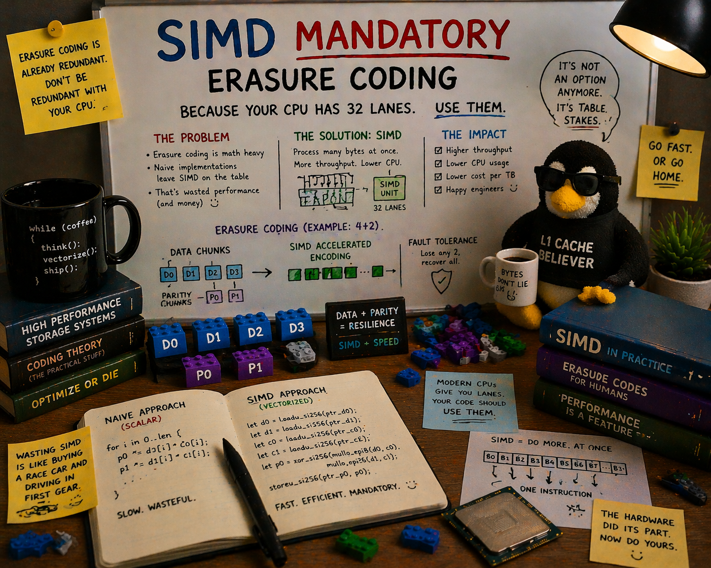
Every production erasure coding library ships a scalar fallback path. This is treated as a virtue: “works on any hardware.” It’s actually a liability. A scalar Reed-Solomon encoder on a single core tops out around 200 MB/s. A single NVMe Gen4 drive does 7 GB/s sequential reads. Your erasure coding layer can’t keep up with one drive, let alone twenty-four. SIMD isn’t an optimization for EC. It’s a structural requirement.
The Math That Makes This Unavoidable
Erasure coding in storage systems is almost universally Reed-Solomon over GF(2^8), the Galois field with 256 elements. Every byte value (0x00 through 0xFF) is an element of this field. Addition is XOR. Multiplication is polynomial multiplication modulo an irreducible polynomial (typically x^8 + x^4 + x^3 + x^2 + 1, the same one AES uses).
Reed-Solomon encoding works like this: you take K data shards and compute M parity shards by multiplying each data shard by a row of a coding matrix over GF(2^8). The computation is:
parity[j][i] = Σ (matrix[j][k] * data[k][i]) for k = 0..K-1Where every * is a GF(2^8) multiply and every Σ is a GF(2^8) add (XOR). For a 4+2 scheme (4 data shards, 2 parity shards), encoding one byte position requires 8 GF multiplies and 6 XORs. For a shard of 1 million bytes, that’s 8 million GF multiplies.
Why GF(2^8) Multiply Is Expensive in Scalar
Scalar GF(2^8) multiplication on a general-purpose CPU requires one of two approaches:
Lookup table. Precompute a 256x256 multiplication table (64 KB), then each multiply is a table lookup. The problem: 64 KB doesn’t fit in L1 cache (typically 32-48 KB). Under sustained encoding with random data, you get constant L1 cache misses. Measured throughput: 150-300 MB/s on modern x86 cores, depending on data patterns and cache behavior.
Log/exp table. Convert to logarithms in GF(2^8) (a 256-byte table), add, convert back via antilog (another 256-byte table). Two lookups plus an add and a modular reduction. Both tables fit in L1, but each multiply now costs 4-5 dependent memory accesses. Measured throughput: 200-400 MB/s.
Either way, scalar GF multiplication is fundamentally slow because it’s memory-bound, not compute-bound. The CPU has plenty of ALU cycles to spare, but it’s waiting on table lookups.
Why SIMD Transforms the Problem
SIMD doesn’t just do the same thing faster. It transforms GF multiplication from a memory-bound lookup into a compute-bound parallel operation. The technique is called split table multiplication with SSSE3/AVX2 shuffles, and it’s brilliantly simple.
The core insight: any GF(2^8) multiply by a constant c can be decomposed into two 4-bit lookups:
c * x = table_lo[x & 0x0F] XOR table_hi[x >> 4]Where table_lo and table_hi are 16-entry tables (one for each nibble value). Each table has 16 entries of 1 byte = 16 bytes. Sixteen bytes is exactly the width of an SSE register.
The PSHUFB (Packed Shuffle Bytes) instruction takes a 16-byte register of table entries and a 16-byte register of indices, and returns a 16-byte register of looked-up values. It’s a 16-way parallel table lookup that executes in a single clock cycle.
┌─────────────────────────────────────────────┐
│  One PSHUFB instruction:                    │
│  Input:  16 bytes of data (low nibbles)     │
│  Table:  16 bytes of GF multiply results    │
│  Output: 16 GF multiplications in 1 cycle   │
├─────────────────────────────────────────────┤
│  Two PSHUFBs + one PXOR:                    │
│  = 16 full GF(2^8) multiplications          │
│  = 3 instructions, ~1-2 clock cycles        │
└─────────────────────────────────────────────┘
With AVX2 (256-bit registers), you get 32 GF multiplies per PSHUFB. With AVX-512, 64. Each instruction has a throughput of one per clock on modern CPUs (Zen 4, Golden Cove).
This is why the throughput gap is so large. The scalar path does one GF multiply per 3-5 cycles (table lookup latency). The SIMD path does 32-64 GF multiplies per 3 cycles (two shuffles plus XOR). That’s a 50-100x improvement per core.
The Throughput Gap: Numbers That Should Scare You
Here are measured encode throughput numbers for a 4+2 Reed-Solomon configuration on a single core:
| Implementation | ISA | Throughput (GB/s) | Notes |
|---|---|---|---|
| Scalar (log/exp table) | Generic | 0.2-0.4 | L1 cache dependent |
| SSSE3 (128-bit PSHUFB) | x86-64 | 2.0-3.0 | 2009+ CPUs |
| AVX2 (256-bit VPSHUFB) | x86-64 | 6.0-9.0 | 2013+ CPUs |
| AVX-512 (512-bit VPSHUFB) | x86-64 | 12.0-18.0 | Xeon, EPYC |
| NEON (128-bit TBL) | AArch64 | 3.0-6.0 | Apple M-series, Graviton |
| SVE/SVE2 (variable width) | AArch64 | 5.0-10.0 | Graviton 3+, Neoverse V2 |
Throughput = input data processed per second. Sources: ISA-L benchmarks, reed-solomon-simd benchmarks, klauspost/reedsolomon Go benchmarks.
Now compare with what you need to keep up:
| Drive Configuration | Sequential Read Throughput | EC Encode Required |
|---|---|---|
| 1x NVMe Gen4 | 7 GB/s | 7 GB/s |
| 1x NVMe Gen5 | 14 GB/s | 14 GB/s |
| 4x NVMe Gen4 | 28 GB/s | 28 GB/s |
| 24x NVMe Gen4 | 168 GB/s | 168 GB/s |
| 32x NVMe Gen5 | 448 GB/s | 448 GB/s |
A scalar encoder at 300 MB/s cannot keep up with a single NVMe Gen4 drive. You’d need 23 dedicated CPU cores just for EC encoding to match one 7 GB/s drive. For a 24-drive system, you’d need 560 cores. For scalar encoding. This isn’t a “nice to have faster” situation. Scalar EC at NVMe line rate is a mathematical impossibility.
With AVX2, a single core encodes at ~8 GB/s, enough to keep up with one Gen4 drive. Four cores cover a 24-drive system at typical write rates. That’s the difference between “dedicating your entire CPU budget to erasure coding” and “EC is a rounding error in your CPU utilization.”
How Production Systems Do It
Nobody ships scalar EC in production. Let me walk through what the major storage systems actually use.
Intel ISA-L (Intelligent Storage Acceleration Library)
The gold standard. ISA-L is Intel’s open-source library that provides SIMD-optimized erasure coding (plus CRC, compression, and crypto). Ceph uses it as the primary EC engine. HDFS uses it via Intel’s native EC codec. DAOS runs it natively.
ISA-L detects CPU features at runtime (CPUID) and dispatches to the fastest available kernel: AVX-512 > AVX2 > SSSE3 > SSE2. On a Sapphire Rapids Xeon, ISA-L’s ec_encode_data hits 15+ GB/s per core for typical RS configurations.
The downside: ISA-L is C code with handwritten assembly for each ISA target. Integrating it into a Rust or Go storage system means crossing an FFI boundary.
klauspost/reedsolomon (Go)
The de facto standard for EC in the Go ecosystem. Used by several major object storage systems. It uses Go assembly (.s files) with AVX2 and NEON kernels. No scalar fallback in the hot path. The library detects SIMD support at init time and panics (or falls back to a dramatically slower pure-Go path) if the minimum ISA isn’t available.
Performance: 8-12 GB/s per core on AVX2. Competitive with ISA-L despite being Go assembly rather than C/intrinsics.
Klaus Post also wrote leopard-rs, a library for Leopard-RS (a different EC algorithm based on FFTs over GF(2^16)), which achieves even higher throughput for configurations with many parity shards.
reed-solomon-simd (Rust)
Pure Rust, no C dependencies, no handwritten assembly. It uses Rust’s std::arch SIMD intrinsics (AVX2 _mm256_shuffle_epi8, NEON vqtbl1q_u8) to implement the split-table GF multiply technique. Runtime detection via the cpufeatures crate.
Performance: 6-10 GB/s per core on AVX2, 3-6 GB/s on NEON. Slightly behind ISA-L on peak throughput, but the entire implementation is memory-safe Rust (the SIMD intrinsics are unsafe, but they’re encapsulated in a well-tested library, not scattered through application code).
The API is clean:
// Encode: data shards in, parity shards out
let parity = reed_solomon_simd::encode(
    data_shards,    // K = 8
    parity_shards,  // M = 4
    &data_slices,   // &[&[u8]], K slices of equal length
)?;

// Decode: any K of K+M shards in, missing shards out
let restored = reed_solomon_simd::decode(
    data_shards,
    parity_shards,
    surviving_data.iter().map(|(idx, data)| (*idx, data.as_slice())),
    surviving_parity.iter().map(|(idx, data)| (*idx, data.as_slice())),
)?;
No configuration for SIMD mode. No feature flags. It detects what your CPU supports and uses the fastest available path. If your CPU has SSSE3 (any x86-64 CPU made after 2008), it uses SIMD. If you’re on ARM with NEON (any ARMv8 CPU, so any Apple Silicon, any Graviton, any Ampere Altra), it uses SIMD.
The Fallback Trap
So if every production library uses SIMD, why do they all ship scalar fallback code?
The usual justifications:
“CI/CD environments might not have SIMD.” This is the most common excuse and the weakest. CI runners on GitHub Actions, GitLab CI, and every major cloud provider run on x86-64 CPUs with at least AVX2 (Haswell-era, 2013). ARM CI runners have NEON. If your CI environment doesn’t support SSSE3, your CI environment is running on a CPU from 2007 and you have bigger problems.
“Portability to exotic architectures.” Fair enough for a general-purpose library. Not relevant for a storage system. Storage systems run on x86-64 or AArch64. Period. Nobody is deploying petabyte-scale object storage on MIPS, RISC-V (yet), or PowerPC. When RISC-V storage deployments become real, they’ll have the V (vector) extension, which supports the same shuffle-based GF multiply technique.
“Graceful degradation is better than hard failure.” This sounds reasonable until you think about what “graceful degradation” means for EC. At 300 MB/s encode throughput, your 24-NVMe storage node has silently become a 300 MB/s system. That’s not graceful degradation. That’s a 50x performance cliff that no monitoring dashboard will explain because the system is “working.” A hard failure at startup with a clear error message (“SIMD required: AVX2 or NEON not detected”) is infinitely more debuggable than mysterious throughput collapse.
“The compiler will auto-vectorize it.” No, it won’t. Auto-vectorization works on simple loops with straightforward arithmetic: add, multiply, compare. GF(2^8) multiplication is not straightforward arithmetic. It’s polynomial multiplication modulo an irreducible polynomial. The compiler doesn’t know about carry-less multiply. It doesn’t know that XOR is addition in GF(2). It doesn’t know that the nibble-split lookup trick transforms a memory-bound computation into a compute-bound one. I’ve looked at the codegen from rustc and gcc with -O3 -mavx2 for a scalar GF multiply loop. Neither compiler vectorizes it. They emit byte-at-a-time table lookups, exactly as written.
The right answer: SIMD should be a hard requirement at startup. Check CPUID, verify AVX2 (x86) or NEON (ARM), and refuse to start if neither is present. Print a clear error. Don’t silently fall back to a path that makes your system 50x slower.
Cauchy vs Vandermonde: The Matrix Matters
Not all Reed-Solomon implementations are equal, even at the same SIMD width. The choice of coding matrix affects how much work the SIMD units actually do.
Vandermonde Matrices
Classical Reed-Solomon uses a Vandermonde matrix (powers of generator elements):
┌                           ┐
│  1    1    1    1   ...    │
│  α⁰   α¹   α²   α³  ...  │
│  α⁰   α²   α⁴   α⁶  ...  │
│  α⁰   α³   α⁶   α⁹  ...  │
└                           ┘
Each matrix entry is a GF(2^8) element. Computing parity requires multiplying each data byte by the matrix entry and XORing the results. With SIMD, each matrix-entry multiply uses the split-table technique (2 shuffles + 1 XOR per multiply).
For M parity shards and K data shards, each byte position requires MK GF multiplies = MK * (2 shuffles + 1 XOR) = 3MK SIMD instructions.
Cauchy Matrices
Cauchy matrices over GF(2^8) have a useful property: they can be decomposed into binary matrices (over GF(2)) through a process called “binary extension.” Each GF(2^8) multiply becomes 8x8 XOR operations on individual bits.
Many entries in the binary-extended Cauchy matrix are 0 or 1. Zero entries skip computation entirely. One entries are just XOR (no multiply needed). Only entries that are neither 0 nor 1 require a GF multiply.
In practice, a well-constructed Cauchy matrix reduces the total operation count by 20-40% compared to Vandermonde for typical storage configurations (K=4-16, M=2-4). More importantly, the operations that remain are predominantly XORs, which are cheaper than shuffles on all SIMD architectures (XOR has higher throughput and lower latency than PSHUFB on Intel cores).
Who uses what:
| Library | Matrix Type | Notes |
|---|---|---|
| ISA-L | Cauchy | Optimized binary Cauchy with XOR reduction |
| klauspost/reedsolomon | Cauchy (via Leopard-like optimization) | Default for new encoders |
| reed-solomon-simd | Cauchy | Binary extension with XOR optimization |
| Jerasure | Both (configurable) | Cauchy recommended |
The industry has converged on Cauchy. If someone tells you their RS implementation uses a Vandermonde matrix, they’re leaving 20-40% of SIMD throughput on the table.
ARM Isn’t x86-Lite: NEON and SVE Are Real
A common misconception: SIMD-optimized EC is “an Intel thing” and ARM systems get scalar fallbacks. This hasn’t been true since 2011.
ARM NEON provides 128-bit SIMD with the TBL instruction, which is functionally equivalent to x86’s PSHUFB for table lookups. Every ARMv8-A CPU has NEON. That includes:
- Apple M1/M2/M3/M4. All Mac and iPad chips since 2020.
- AWS Graviton 2/3/4. The most popular ARM server platform.
- Ampere Altra/AmpereOne. Up to 192 cores, designed for cloud.
- NVIDIA Grace. The CPU half of Grace Hopper superchip.
NEON EC throughput is typically 3-6 GB/s per core. On a 128-core Ampere Altra, that’s 384-768 GB/s aggregate EC throughput across all cores. Plenty for even the densest NVMe configurations.
ARM SVE (Scalable Vector Extension) goes further. SVE vector widths are implementation-defined (128 to 2048 bits), and SVE2 (mandatory in ARMv9) adds cryptographic and per-lane operations that can further accelerate GF arithmetic. AWS Graviton 3 has SVE with 256-bit vectors; Neoverse V2 (Graviton 4) has the same. SVE EC implementations are still maturing, but early benchmarks show 30-50% throughput improvement over NEON.
If you’re designing a storage system in 2026 that runs on ARM (and you should be, given Graviton’s price-performance advantage), your EC library needs NEON support as a first-class citizen, not an afterthought. The major libraries (ISA-L, klauspost/reedsolomon, reed-solomon-simd) all provide it.
The Decode Side: Even More SIMD-Critical
Everything above focuses on encode throughput. Decode (reconstruction from partial shards after a failure) is worse.
RS decode requires:
-
Matrix inversion. Given the set of K surviving shards (out of K+M), compute the inverse of the corresponding K-row submatrix of the coding matrix. This is O(K^3) GF multiplies. For K=16, that’s 4,096 GF multiplies. Expensive, but it’s a one-time cost per reconstruction.
-
Matrix-vector multiplication. Multiply each surviving shard by the inverted matrix to recover the missing shards. This is the same structure as encoding: M_missing * K GF multiplies per byte position.
The practical effect: decode throughput is roughly (K / M_missing) * encode throughput for the matrix-vector phase, but the constant factor is larger because the inverted matrix entries are “random” GF elements (unlike the structured Cauchy matrix used for encoding), which means fewer zero/one optimizations.
Decode throughput for 8+4 with 4 shards lost, AVX2:
| Library | Decode Throughput (GB/s per core) |
|---|---|
| ISA-L | 3.5-5.0 |
| klauspost/reedsolomon | 3.0-4.5 |
| reed-solomon-simd | 2.5-4.0 |
| Scalar fallback | 0.08-0.15 |
Scalar decode is even slower than scalar encode because the inverted matrix has worse cache behavior. At 100 MB/s, reconstructing a single 30 TB drive takes 83 hours. With AVX2 at 4 GB/s on 4 dedicated cores, it’s 2 hours. That’s the difference between “your data is at risk for 3.5 days” and “your data is at risk for 2 hours.”
In a system with 24 drives where the probability of a second drive failure increases with time, reconstruction speed directly determines your MTTDL (Mean Time To Data Loss). Scalar decode doesn’t just make things slower. It makes your data less durable.
What “Mandatory” Looks Like in Practice
I’ve argued that SIMD should be a hard requirement for EC. Here’s what that means concretely in a storage system’s codebase.
Startup Check
fn verify_simd_support() -> Result<(), StartupError> {
    #[cfg(target_arch = "x86_64")]
    {
        if !std::is_x86_feature_detected!("avx2") {
            return Err(StartupError::UnsupportedHardware(
                "AVX2 required for erasure coding. \
                 CPU does not support AVX2 (requires Haswell/2013 or later)."
                    .into(),
            ));
        }
    }

    #[cfg(target_arch = "aarch64")]
    {
        // NEON is mandatory in ARMv8-A. If we're on AArch64, we have it.
        // No check needed.
    }

    #[cfg(not(any(target_arch = "x86_64", target_arch = "aarch64")))]
    {
        return Err(StartupError::UnsupportedHardware(
            "Unsupported architecture. Erasure coding requires \
             x86-64 (AVX2) or AArch64 (NEON)."
                .into(),
        ));
    }

    Ok(())
}
This runs once at process startup, before any data is written. If the check fails, the process prints a clear error and exits. No silent degradation. No surprise 50x slowdown three months later when someone replaces a drive and triggers a rebuild.
Library Choice
Use a library that is SIMD-first, not SIMD-optional:
- reed-solomon-simd (Rust): automatically detects and uses the fastest available ISA. The library name literally has “simd” in it.
- ISA-L (C): the “ISA” stands for “Intelligent Storage Acceleration.” SIMD is the product, not a feature.
- klauspost/reedsolomon (Go): uses Go assembly with SIMD kernels. The scalar path exists but is documented as “do not use in production.”
No Feature Gate for Scalar
Don’t provide a --allow-scalar-ec flag. Don’t add a disable-simd feature in your Cargo.toml. Every escape hatch becomes someone’s production configuration. The moment you add a scalar option, someone will enable it “just for testing” and forget to disable it. A year later, you’re debugging why a customer’s rebuild is taking 4 days and the answer is a flag in a config file nobody remembers setting.
The Counter-Arguments (And Why They’re Wrong)
“But what about testing on my laptop?”
Your laptop has AVX2. Every Intel laptop since Haswell (2013) and every AMD laptop since Excavator (2015) supports AVX2. Every Apple Silicon Mac has NEON. If you’re developing a storage system on a laptop that doesn’t support SSSE3, you’re working on hardware that’s old enough to vote.
”What about Docker / QEMU / emulated environments?”
Docker passes through the host CPU’s SIMD support. If your Docker host has AVX2, containers see AVX2. QEMU with KVM also passes through host SIMD. QEMU in full emulation mode doesn’t, but nobody runs production storage in full CPU emulation.
”What about WASM?”
WASM has SIMD128, which is equivalent to SSE2/NEON (128-bit vectors). This is enough for PSHUFB-based GF multiply. Regardless, nobody is running erasure coding in WASM in production storage. This is a future concern, not a present one.
”The throughput gap will shrink as CPUs get faster.”
The gap scales with vector width. As CPUs add wider SIMD (AVX-512 was 512 bits, ARM SVE can be up to 2048 bits), the SIMD path gets proportionally faster. The scalar path doesn’t. The gap is widening, not shrinking.
A Real-World Pipeline
Here’s what the data flow looks like in a SIMD-mandatory storage system for a 100 MB PUT with 8+4 erasure coding:
Client sends 100 MB object
    ↓
Compress (LZ4, ~2 GB/s)                    → 60 MB compressed
    ↓
Encrypt (AES-256-GCM, ~4 GB/s per core)    → 60 MB + 16-byte tags
    ↓
EC Encode (reed-solomon-simd, AVX2)
  Split: 60 MB / 8 shards = 7.5 MB/shard
  Encode: 4 parity shards                  → 12 shards × 7.5 MB
  Time: ~8 ms (single core, 8 GB/s)
    ↓
BLAKE3 checksum per shard (~6 GB/s)         → 12 × 32-byte hashes
    ↓
Write 12 shards to NVMe (parallel)          → 90 MB total, ~13 ms at 7 GB/s
    ↓
Write metadata (FlatBuffer, <512 bytes)     → <1 ms
    ↓
Total wall time: ~35 ms
EC encoding at 8 ms is 23% of the total pipeline. Acceptable. With scalar encoding at 300 MB/s, the encode step alone would take 200 ms, ballooning total wall time to 225 ms and making EC the dominant bottleneck. The rest of the pipeline (compress, encrypt, hash, write) is fast. EC is only fast if you use SIMD.
The Industry Has Already Decided
Look at the actual production deployments:
| System | EC Library | SIMD Required | Scalar Fallback |
|---|---|---|---|
| Ceph | ISA-L / Jerasure | Yes (ISA-L default) | Jerasure as fallback |
| HDFS | ISA-L (native codec) | Yes | Java fallback (10x slower) |
| DAOS | ISA-L | Yes | None |
Every system that matters uses SIMD for erasure coding. The ones that provide scalar fallbacks document them as “not for production use.” HDFS’s Java EC codec is so slow that the documentation explicitly recommends the ISA-L native codec for anything beyond testing.
The debate isn’t “should we use SIMD for EC?” That question was answered a decade ago. The real question is “should we even compile the scalar path?” And my answer is no. Drop it. Ship SIMD-only. Your binary gets smaller, your test matrix gets simpler, and nobody accidentally deploys on a path that turns their storage system into a bottleneck.
Conclusion
Erasure coding is GF(2^8) arithmetic at scale. GF(2^8) arithmetic is a shuffle-table computation that maps perfectly to SIMD instructions. Every modern CPU (x86-64 since 2008, AArch64 since 2011) has the SIMD instructions needed. The throughput gap between scalar and SIMD is 30-100x. NVMe drives are fast enough that scalar EC can’t keep up with a single drive, let alone a chassis full of them.
The entire history of storage EC points in one direction: SIMD isn’t optional. ISA-L, klauspost/reedsolomon, and reed-solomon-simd all implement the same split-table GF multiply technique, all use the same PSHUFB/TBL instruction, and all achieve throughput that makes EC a small fraction of the I/O pipeline instead of the bottleneck.
Ship your storage system with a CPUID check at startup. Require AVX2 on x86, NEON on ARM. Print a clear error if neither is present. Don’t provide a scalar fallback, don’t provide a flag to skip the check, and don’t apologize for it. Any CPU that doesn’t support SSSE3 is old enough that it shouldn’t be running a storage system handling production data.
Your drives are fast. Your network is fast. Your compression is fast. Make sure your erasure coding is, too.
ISA-L source and benchmarks from Intel’s ISA-L repository. klauspost/reedsolomon from Klaus Post’s GitHub. reed-solomon-simd from crates.io. GF(2^8) split-table multiply technique described in James Plank’s FAST 2013 tutorial. Cauchy RS optimization from Plank and Xu, “Optimizing Cauchy Reed-Solomon Codes for Fault-Tolerant Storage Applications”. NVMe Gen4/Gen5 throughput from NVM Express specification 2.0. NEON shuffle instruction reference from ARM Architecture Reference Manual. Ceph EC configuration from Ceph documentation. HDFS native codec recommendation from Apache HDFS EC documentation.
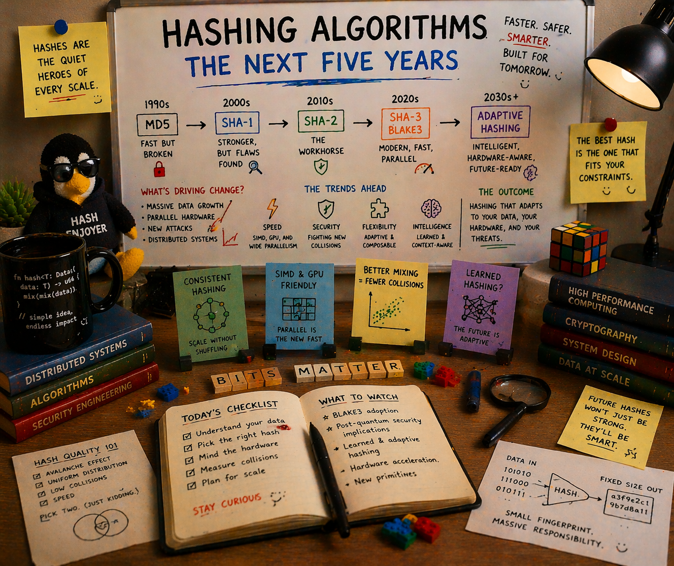
A practitioner’s guide to CRC32, MD5, SHA-256, XXHash, SipHash, HighwayHash, BLAKE2, and BLAKE3. What each was designed for, where each breaks down, and which one you should bet your architecture on for the next five years.
Why This Matters More Than You Think
Every storage system makes a hashing decision early in its life, and that decision haunts it forever.
ZFS chose fletcher4 in 2005, a fast, non-cryptographic checksum that can’t detect adversarial corruption. Twenty years later, OpenZFS is backporting BLAKE3 support because the original choice wasn’t strong enough. btrfs shipped with CRC32C, giving you 32 bits of collision resistance in a world where a single NVMe drive holds 30 TB. HDFS used CRC32C and never offered anything else. AWS S3 used MD5 for ETags and spent nearly two decades unable to change it. Only in 2024 did they finally default to CRC64-NVME.
MinIO chose HighwayHash in 2017. It was the right call at the time: blazing fast, keyed integrity, perfect for bitrot detection. The hash field in 2026 looks nothing like 2017.
The hash you choose determines your collision resistance, your throughput ceiling, your regulatory compliance story, your post-quantum readiness, and (if you’re building something meant to last) whether your integrity guarantees will still hold in 2031.
This is the guide I wish I’d had before making hashing decisions at three different storage companies.
The Contenders
Let me lay out the field. Nine algorithms, three categories, one question: which one deserves to be the default for the next generation of object storage?
The Non-Cryptographic Speed Demons
| Algorithm | Throughput (GB/s) | Output | Collision Bits | Year |
|---|---|---|---|---|
| CRC32C (SSE4.2) | ~5.7 | 32-bit | 32 | 1975 |
| CRC32C (AVX-512 VPCLMULQDQ) | ~97 | 32-bit | 32 | 2019+ |
| XXHash3 (64-bit) | ~31.5 | 64-bit | 64 | 2019 |
| XXH128 | ~29.6 | 128-bit | 128 | 2019 |
The Keyed PRFs (Pseudorandom Functions)
| Algorithm | Throughput (GB/s) | Output | Security Model | Year |
|---|---|---|---|---|
| SipHash-2-4 | ~2.0 | 64-bit | Keyed PRF | 2012 |
| SipHash-1-3 | ~3.8 | 64-bit | Keyed PRF (reduced) | 2012 |
| HighwayHash-256 (AVX2) | ~10-12 | 256-bit | Keyed PRF | 2016 |
The Cryptographic Hashes
| Algorithm | Throughput (GB/s) | Output | Collision Bits | FIPS | Year |
|---|---|---|---|---|---|
| MD5 | ~0.69 | 128-bit | 0 (broken) | Disallowed | 1992 |
| SHA-256 (no SHA-NI) | ~0.22 | 256-bit | 128 | Yes | 2001 |
| SHA-256 (SHA-NI hw) | ~1.5 | 256-bit | 128 | Yes | 2001 |
| SHA-3-256 | ~0.55 | 256-bit | 128 | Yes | 2015 |
| BLAKE2b-256 | ~0.75 | 256-bit | 128 | No | 2012 |
| BLAKE3 (AVX2) | ~6.4 | 256-bit | 128 | No | 2020 |
| BLAKE3 (AVX-512) | ~8.4 | 256-bit | 128 | No | 2020 |
| BLAKE3 (multi-threaded) | ~15.8 | 256-bit | 128 | No | 2020 |
Benchmarks: single-threaded on modern x86-64 (Cascade Lake, Ice Lake, Sapphire Rapids class), large messages (≥4 KB). Sources: BLAKE3 paper, xxHash repo, Google HighwayHash repo, btrfs wiki, Joey Lynch’s hash benchmarks.
Look at that table carefully. BLAKE3 on AVX2 delivers 6.4 GB/s. Cryptographic-strength hashing, at a speed nobody would have believed five years ago. 4x faster than SHA-256 with hardware acceleration. 8x faster than BLAKE2b. 30x faster than SHA-256 in software.
And it’s the only cryptographic hash in the table that gets faster when you throw more cores at it.
Algorithm by Algorithm: The Full Story
CRC32C: The Honest Checksum
What it is. A 32-bit cyclic redundancy check using the Castagnoli polynomial (0x1EDC6F41), hardware-accelerated via Intel’s SSE4.2 CRC32 instruction since Nehalem (2008).
What it’s good for. Detecting random bit errors in transit: network corruption, memory errors, storage media degradation. CRC32C is the workhorse of error detection in databases (RocksDB, ScyllaDB), network protocols (iSCSI, gRPC), and filesystems (btrfs default).
What it can’t do. Anything adversarial. CRC32C has exactly 32 bits of collision resistance, which means a brute-force collision takes roughly 2^16 = 65,536 attempts. An attacker with a laptop can forge a collision in milliseconds. It cannot detect intentional tampering. It cannot serve as a content address. It cannot provide deduplication safety.
The hardware acceleration story is remarkable. On Sapphire Rapids with AVX-512 VPCLMULQDQ, CRC32C hits 97 GB/s, faster than DRAM bandwidth on most systems. But speed doesn’t compensate for 32 bits of output. A 30 TB NVMe drive has roughly 2^34 sectors; with 32-bit checksums, you expect at least one undetected collision by random chance once the drive is ~16% full. For petabyte-scale storage, CRC32C is structurally inadequate.
Who still uses it. btrfs (default), HDFS, RocksDB, gRPC. These are legacy choices that made sense when CPU time was expensive and disks were small.
Verdict. Use it for wire-level error detection where you also have a stronger integrity check at rest. Never use it as your only defense against corruption.
MD5: The Walking Dead
What it is. A 128-bit cryptographic hash designed by Ron Rivest in 1991. Merkle-Damgard construction, 64 rounds.
Why it’s still everywhere. AWS S3 defined ETags as MD5 digests in 2006. Every S3 client in the world computes MD5 on upload. Every S3 server in the world returns MD5 in the ETag header. Changing this required nearly two decades of backwards compatibility work. AWS only defaulted to CRC64-NVME for new buckets in 2024.
Why it must die. MD5 has been cryptographically broken since 2004. Wang et al. demonstrated collision attacks that year. By 2008, researchers demonstrated chosen-prefix collisions against X.509 certificates. Today, a full MD5 collision takes under a second on a single core.
The only reason to compute MD5 in 2026 is S3 API compatibility. MinIO’s brilliant hack, the md5-simd library that uses AVX-512 to compute 16 MD5 hashes simultaneously, pushes aggregate throughput to 17 GB/s. But that’s 17 GB/s of effort wasted on a broken algorithm, spent purely because AWS defined the API 20 years ago.
Verdict. Compute it for ETags if you must speak S3. Never use it for integrity, addressing, or deduplication.
SHA-256: The Regulatory Standard
What it is. The 256-bit member of the SHA-2 family (FIPS 180-4), designed by the NSA. Merkle-Damgard construction, 64 rounds.
Performance:
- Software: ~220 MB/s, painfully slow for storage workloads
- SHA-NI hardware (all modern x86 since 2017): ~1.5 GB/s, usable but not fast
- AVX-512 multi-buffer (8 parallel streams): ~3.5 GB/s aggregate
The FIPS advantage is real. SHA-256 is the only hash function in this comparison that is approved under FIPS 180-4 and FIPS 140-3. If your storage system serves U.S. government agencies, healthcare organizations under HIPAA, financial institutions, or defense contractors, SHA-256 is not optional. It’s mandated. No amount of BLAKE3 benchmarks changes a compliance requirement.
The performance disadvantage is also real. At 1.5 GB/s with SHA-NI, SHA-256 is 4x slower than BLAKE3 on AVX2 and 55x slower than BLAKE3 multi-threaded. On a storage node processing 10 million objects per day, that’s the difference between hashing being invisible overhead and hashing being a measurable bottleneck.
Who uses it. ZFS (optional), btrfs (optional), git (migrating from SHA-1), Bitcoin, TLS, Docker content addressing, AWS SigV4 authentication.
Verdict. The compliance hash. Use it when regulations demand it. Don’t use it by default when you have better options. You’re paying a 4-7x performance tax for a NIST stamp.
SHA-3 (Keccak): The Insurance Policy Nobody Uses
What it is. The winner of NIST’s SHA-3 competition (2012), standardized as FIPS 202. Sponge construction based on the Keccak permutation, fundamentally different from SHA-2’s Merkle-Damgard design.
Performance. ~0.55 GB/s on modern x86-64. That’s slower than SHA-256 with SHA-NI, and there are no hardware acceleration instructions for SHA-3 on any current x86 CPU. Intel has shown no interest in adding them.
Why it exists. NIST wanted a backup in case SHA-2 was broken. SHA-3’s sponge construction means a break in SHA-2 wouldn’t imply a break in SHA-3. It’s also immune to length-extension attacks (unlike SHA-256), which matters for MAC constructions but is irrelevant for storage checksums.
Why nobody uses it for storage. It’s slower than SHA-256 on hardware-accelerated x86, offers the same 128-bit collision resistance for SHA3-256, and has no unique advantage for integrity checking workloads. The KangarooTwelve variant (reduced-round Keccak with tree hashing) is significantly faster but isn’t FIPS-standardized.
Verdict. Theoretically interesting, practically irrelevant for storage. Keep it in your regulatory toolkit in case SHA-2 is ever compromised. Don’t build a storage system around it.
XXHash3: The Speed King
What it is. Yann Collet’s non-cryptographic hash, designed purely for speed. 64-bit and 128-bit variants.
Performance. 31.5 GB/s on an i7-9700K with SSE2. At that speed, XXHash3 is faster than DRAM bandwidth. The benchmark data lives in L3 cache. In real-world scenarios where data streams from memory, XXHash3 is effectively memory-speed limited, not compute-limited.
What it gives you. Maximum throughput for non-adversarial checksumming. If your threat model is exclusively random bit errors (cosmic rays, media degradation, controller bugs), and you need maximum performance, XXHash3 is the answer.
What it can’t give you. Any cryptographic guarantee whatsoever. XXHash3 is not designed to resist adversarial collisions, preimage attacks, or second-preimage attacks. A determined attacker can construct collisions efficiently. It is not a substitute for a cryptographic hash in any scenario where an adversary might modify data.
Who uses it. btrfs (xxhash64 option, recommended for performance-sensitive workloads), Ceph (internally), various databases for page checksums, data pipelines for deduplication of trusted data.
Verdict. The best non-cryptographic hash available. Use it for in-process checksums, page verification, and integrity checks within a trusted boundary. Never use it as the sole integrity mechanism for data at rest in a storage system exposed to untrusted clients.
SipHash: The Hash Table Protector
What it is. A keyed PRF (pseudorandom function) designed by Jean-Philippe Aumasson and Daniel J. Bernstein specifically to protect hash tables against algorithmic complexity attacks (HashDoS).
Performance. ~2 GB/s for SipHash-2-4, ~3.8 GB/s for the reduced SipHash-1-3. Optimized for short inputs (8-64 bytes) rather than bulk data.
Why it matters. SipHash is the default hasher in Rust’s standard library HashMap (SipHash-1-3) and Python’s dict (SipHash-2-4). It’s why modern languages are immune to the 2011 HashDoS attacks that took down PHP, Java, and Ruby web servers.
Why it doesn’t matter for storage. SipHash is designed for short, in-memory keys. Its per-byte cost is too high for multi-megabyte objects, and it requires a secret key, making it unsuitable for content addressing.
Verdict. Essential for hash tables. Irrelevant for storage integrity. You’ll use it indirectly through Rust’s HashMap, but never as a storage checksum.
HighwayHash: The Keyed Speedster
What it is. A SIMD-accelerated keyed pseudorandom function developed at Google by Jan Wassenberg and Jyrki Alakuijala (2016). Designed to be the fastest hash that still provides strong integrity guarantees when keyed with a secret 256-bit key.
Performance. ~10-12 GB/s with AVX2. MinIO’s Go implementation achieves similar numbers on Skylake and later. All three output sizes (64, 128, 256 bit) run at the same speed; the core computation is identical, and only the output extraction differs.
How it works. HighwayHash’s permutation is designed around SIMD instructions natively. Instead of computing scalar operations and hoping the compiler auto-vectorizes (it won’t), the algorithm’s internal state maps directly onto AVX2 lanes. Four 64-bit multiplies feed into a mixing step that uses vector addition and rotation. The result is a hash that runs at hardware speed by design, not by optimization.
The typical deployment pattern is bitrot detection in object storage: compute HighwayHash on write, store it alongside the data, verify on every read. Because it runs at 10+ GB/s, verification adds no measurable latency even on fast NVMe drives. If a shard fails verification, the storage system reconstructs from erasure-coded parity and heals the corrupted copy automatically. This inline-verify-and-heal loop is only practical because the hash is fast enough to run on every I/O without becoming a bottleneck.
The limitation:
HighwayHash is a keyed PRF, not a general-purpose cryptographic hash. This means:
- It requires a secret key. Without the key, you can’t verify the hash. This makes it useless for content addressing, deduplication across trust boundaries, and public integrity verification.
- It’s not a collision-resistant hash. The security claim is PRF security under the key. Given the key, an attacker still can’t forge a valid hash. But unkeyed collision resistance (the property you need for content addressing) is not claimed and not proven.
- It hasn’t received deep cryptanalysis. Compared to the SHA-2/SHA-3/BLAKE families, which have been subjected to decades of international cryptanalytic effort (the SHA-3 competition alone generated thousands of papers), HighwayHash has received relatively modest scrutiny. The design is clever: the permutation uses SIMD instructions directly, avoiding the scalar bottlenecks of traditional ARX constructions. But “clever and fast” is not the same as “deeply analyzed and trusted.”
- It’s architecturally limiting. Because the hash depends on a deployment-wide secret key, you can’t compare hashes across deployments, you can’t publish hashes for third-party verification, and you lose the hash if you lose the key.
Verdict. An excellent choice for keyed integrity checking in a closed system where you control both ends. Not the right foundation for a next-generation storage system that needs content addressing, cross-deployment verification, and post-quantum durability.
BLAKE2: The Bridge Generation
What it is. The successor to BLAKE (a SHA-3 finalist), designed by Jean-Philippe Aumasson, Samuel Neves, Zooko Wilcox-O’Hearn, and Christian Winnerlein. Standardized in RFC 7693. Two variants: BLAKE2b (64-bit optimized, 128-byte blocks) and BLAKE2s (32-bit optimized, 64-byte blocks).
Performance. BLAKE2b at ~750 MB/s is faster than SHA-256 in software but slower than SHA-256 with SHA-NI. The parallel variants (BLAKE2bp, BLAKE2sp) reach ~1.6 GB/s using 4-way or 8-way tree hashing, but this requires committing to a tree mode at the API level.
Legacy. BLAKE2 proved that the BLAKE/ChaCha core (add, rotate, XOR operations) could outperform SHA-256 while maintaining cryptographic security. It earned widespread adoption: WireGuard, libsodium, Zcash, Argon2, IPFS, btrfs (optional). The Rust ecosystem standardized on BLAKE2b through the blake2 crate.
Why BLAKE3 supersedes it. BLAKE3 takes BLAKE2s’s compression function, reduces rounds from 10 to 7, and wraps it in a Merkle tree that enables inherent parallelism without requiring a special API mode. The result: 6.4 GB/s vs. 750 MB/s, an 8.5x speedup over BLAKE2b, using the same fundamental cryptographic core. BLAKE3 is to BLAKE2 what BLAKE2 was to SHA-256: the same security lineage, dramatically better performance.
Verdict. A great hash that served its era well. BLAKE3 is its direct successor in every meaningful dimension: faster, simpler API, built-in parallelism, same security lineage. New systems should use BLAKE3.
BLAKE3: The Future
What it is. A cryptographic hash function built on a Merkle tree of BLAKE2s-derived compressions. Designed by Jack O’Connor, Jean-Philippe Aumasson, Samuel Neves, and Zooko Wilcox-O’Hearn. Released January 2020.
Why it’s different: the architecture.
Every other cryptographic hash in this comparison is inherently serial. SHA-256 processes 64-byte blocks one at a time, where each block’s compression depends on the previous block’s output (Merkle-Damgard chaining). To hash a 1 MB file, you must perform ~16,384 sequential compressions. No amount of SIMD or multi-threading can parallelize this.
BLAKE3 breaks the chain. The input is split into 1,024-byte chunks, each hashed independently. The chunk outputs form the leaves of a binary Merkle tree, and parent nodes combine pairs of children through a single compression call. This structure is embarrassingly parallel at every level:
Input: [chunk₀] [chunk₁] [chunk₂] [chunk₃] [chunk₄] [chunk₅] [chunk₆] [chunk₇]
          ↓        ↓        ↓        ↓        ↓        ↓        ↓        ↓
Level 0:  h₀       h₁       h₂       h₃       h₄       h₅       h₆       h₇
           \      /           \      /           \      /           \      /
Level 1:    h₀₁                h₂₃                h₄₅                h₆₇
              \              /                        \              /
Level 2:       h₀₁₂₃                                  h₄₅₆₇
                    \                              /
Root:                    BLAKE3(input)
SIMD parallelism within a single thread. The BLAKE2s-derived compression uses 32-bit words. An AVX2 register (256 bits) holds 8 x 32-bit values, allowing 8 independent chunk compressions to proceed in lockstep. AVX-512 doubles this to 16 chunks per vector operation. This is why BLAKE3 chose BLAKE2s (32-bit) over BLAKE2b (64-bit) as its base: twice the SIMD parallelism per register width.
| SIMD Level | Register Width | Chunks in Parallel | Input Window |
|---|---|---|---|
| SSE4.1 | 128-bit | 4 chunks | 4 KiB |
| AVX2 | 256-bit | 8 chunks | 8 KiB |
| AVX-512 | 512-bit | 16 chunks | 16 KiB |
| ARM NEON | 128-bit | 4 chunks | 4 KiB |
Multi-threaded parallelism across cores. Because chunks are independent, the Rust implementation supports Rayon-based multithreading (opt-in). On an 8-core machine, BLAKE3 reaches ~15.8 GB/s, hashing faster than most NVMe drives can deliver data. The b3sum CLI tool enables this by default.
Streaming verification. The Merkle tree structure means a receiver can verify chunks incrementally without buffering the entire file. This enables verified streaming downloads, where each chunk can be authenticated independently against the root hash. For a storage system serving 100 GB objects, this is not a nice-to-have. It’s essential.
Extendable output (XOF). BLAKE3 can produce output of any length: 128 bits, 256 bits, 384 bits, or beyond. Shorter outputs are prefixes of longer ones, enabling efficient truncation without recomputation. This matters for storage. You can store a 128-bit truncated hash for ETags, a 256-bit hash for integrity, and a 384-bit hash for post-quantum collision resistance, all from a single computation.
Security:
- Collision resistance: 128 bits (the authors explicitly claim 128-bit security)
- Preimage resistance: 256 bits classically, 128 bits under Grover’s quantum algorithm
- Rounds: 7 (reduced from BLAKE2s’s 10)
- Security margin: Best known attacks reach 2.5 rounds, leaving 64% of rounds untouched, a wider margin than AES-128 (30%) or SHA-256 (28%)
- Cryptanalysis: Zero known attacks better than generic on full 7-round BLAKE3, inheriting the extensive cryptanalytic effort from the BLAKE family during and after the SHA-3 competition
- Side channels: The ARX (add-rotate-XOR) construction is inherently constant-time. No table lookups, no data-dependent branches, no cache-timing vulnerabilities
What it’s missing:
-
FIPS certification. BLAKE3 is not in FIPS 180-4, FIPS 202, or NIST SP 800-140C. An IETF Internet-Draft exists (draft-aumasson-blake3) but it has not been adopted by a working group. For regulated environments, SHA-256 remains the only option.
-
Post-quantum collision resistance at 256-bit output. Under the BHT quantum collision algorithm, a 256-bit hash has ~85-bit collision resistance, below the 128-bit threshold. But BLAKE3’s XOF mode can trivially produce 384-bit or 512-bit digests, restoring full 128-bit quantum collision resistance at negligible cost.
Verdict. BLAKE3 is the biggest jump in hash function design since SHA-256. Cryptographic strength, 6+ GB/s throughput, built-in parallelism, streaming verification, flexible output length. Its only limitation (no FIPS approval) is a regulatory gap, not a technical one.
The Storage System Hash Decision Matrix
Let me cut through the benchmarks and give you the decision framework:
If you need FIPS compliance
SHA-256 with SHA-NI. No choice. It’s slow (1.5 GB/s), it’s from 2001, and it’s the only FIPS 180-4 approved option that’s remotely practical. Budget 4-7x more CPU for hashing than a BLAKE3 system.
If you also need a backup in case SHA-2 is broken: SHA-3-256 (FIPS 202). But you’ll pay an even steeper performance penalty.
If you need maximum non-cryptographic speed
XXHash3 for checksums within a trusted boundary. CRC32C if hardware-accelerated and you only need error detection (not integrity verification against any adversary). Use these for page checksums, network integrity, and in-process verification. Never as the sole integrity mechanism at rest.
If you need keyed integrity (closed system)
HighwayHash-256. This is MinIO’s model: a deployment-wide secret key, HighwayHash per shard, verified on every read. It works well for self-contained systems where you control both writer and reader. Understand the limitation: you can’t do content addressing, cross-deployment verification, or public integrity proofs.
If you’re building new storage infrastructure
BLAKE3. And let me be specific about why:
-
6.4 GB/s single-threaded (AVX2) means hashing is never your bottleneck. Not on NVMe reads, not on 100 GbE network ingestion, not on erasure-coded shard verification.
-
Cryptographic security without the performance tax. You don’t have to choose between “fast but insecure” (XXHash, CRC) and “secure but slow” (SHA-256, SHA-3). BLAKE3 is both.
-
Content addressing is free. Because BLAKE3 is an unkeyed cryptographic hash, the hash of an object is deterministic and verifiable by anyone. This enables deduplication, Merkle-tree-based replication verification, and public integrity proofs. None of which are possible with a keyed PRF like HighwayHash.
-
Streaming verification is built in. The Merkle tree structure means you can verify individual chunks of a multi-gigabyte object without reading the whole thing. For erasure-coded storage where you reconstruct objects from shards, this is essential.
-
Post-quantum ready via XOF. If quantum computing advances threaten 256-bit collision resistance (the BHT algorithm reduces it to ~85 bits), BLAKE3 can output 384-bit or 512-bit digests from the same computation, restoring 128-bit quantum collision resistance.
-
The FIPS gap will close. The IETF draft is in progress. BLAKE3’s lineage (BLAKE was a SHA-3 finalist, BLAKE2 has RFC 7693 and wide deployment) gives it the pedigree for eventual standardization. In the meantime, offer SHA-256 as a configurable fallback for regulated deployments, but make BLAKE3 the default.
The Next Five Years: Where Each Algorithm Lands
Here’s where I think this goes between now and 2031:
Rising
BLAKE3. It will become the default cryptographic hash for new systems. ZFS already supports it (OpenZFS 2.2+). The IETF draft will progress toward RFC status. More storage systems, VCS tools, and integrity frameworks will adopt it as the performance advantage becomes impossible to ignore.
Stable
SHA-256. It’s not going anywhere. FIPS compliance ensures its place. But it will increasingly be the “compliance fallback” rather than the default. New systems will use it only when regulations require it.
XXHash3. Dominant for non-cryptographic checksumming. The ~31 GB/s throughput at 128 bits of output is hard to argue with for trusted-boundary integrity checks.
Declining
HighwayHash. Its niche (keyed integrity faster than any cryptographic hash) has shrunk. At 6.4 GB/s (BLAKE3) vs. 10-12 GB/s (HighwayHash), the speed gap is less than 2x now. And BLAKE3 gives you unkeyed cryptographic strength, content addressing, streaming verification, and post-quantum extensibility on top of that. Existing HighwayHash deployments will keep working fine, but new systems will pick BLAKE3.
BLAKE2. Superseded by BLAKE3 in every dimension. Existing deployments (WireGuard, libsodium, btrfs) will persist, but new projects will use BLAKE3.
MD5. Dead but undead. AWS S3 ETag compatibility will keep it shambling through codebases for another decade. Every S3-compatible server will compute it, and every engineer will wish they didn’t have to.
Extinct (for storage)
CRC32C as a sole integrity mechanism. 32 bits of collision resistance is indefensible at petabyte scale. Systems that use CRC32C today (btrfs default, HDFS) will either add stronger alternatives or accept the risk.
SHA-3 for storage. Without hardware acceleration on x86, it’s slower than SHA-256 with SHA-NI and offers no practical advantage for integrity checking. Its role is NIST insurance, a backup if SHA-2 is ever broken, not a production hash for storage systems.
The Uncomfortable Truth About Hash Migrations
I’ve been through this. At Nexenta, we inherited ZFS’s fletcher4 and lived with its limitations. At my next company, we chose HighwayHash and built an entire integrity architecture around it. Both were the right call when they were made. Both have been overtaken.
The uncomfortable truth is this: you cannot easily change a hash algorithm after deployment. Every stored hash must be recomputed or maintained in parallel. Every client that validates hashes must be updated. Every integrity check that depends on hash comparison must handle the transition period where some objects have old hashes and some have new ones.
This is why the choice matters so much. The hash you choose today is the hash you’ll live with for 5-10 years. Maybe longer. ZFS’s fletcher4 is 20 years old and still the default.
If you’re building something new in 2026, you have the luxury of starting clean. BLAKE3 is the right default. It’s the fastest cryptographic hash available, it scales with your hardware (more SIMD lanes = faster, more cores = faster), it enables streaming verification and content addressing, and it has a clear path to post-quantum safety through its XOF mode.
Offer SHA-256 as a configurable option for FIPS compliance. Compute MD5 for S3 ETag compatibility. But make BLAKE3 the foundation, the hash that holds your data together for the next decade.
The era of choosing between fast and secure is over. BLAKE3 is both.
Hash performance data from the BLAKE3 paper, xxHash repository, Google HighwayHash repository, and Joey Lynch’s hash benchmarks. CRC32C AVX-512 numbers from corsix/fast-crc32. MinIO md5-simd from minio/md5-simd. MinIO HighwayHash from minio/highwayhash. BLAKE3 IETF draft at datatracker.ietf.org. BLAKE3 security analysis and round reduction from BLAKE3 specification. Post-quantum hash security from NIST Post-Quantum Cryptography and the BHT quantum collision algorithm. btrfs checksum benchmarks from the btrfs wiki. SHA-NI performance from Intel SHA Extensions documentation.
Silent data corruption, AI, and why I lost files despite spending years at two data integrity companies.
The Confession
I need to start with a personal story, because it’s the one that made this article real instead of theoretical.
I spent years at Nexenta, the company that built enterprise storage on ZFS, the filesystem famous for one thing above all others: data integrity. ZFS checksums every block. ZFS scrubs detect bit rot before it reaches your applications. ZFS was built, from the ground up, by Jeff Bonwick and Matt Ahrens at Sun Microsystems, specifically because silent data corruption was a known, measured, inevitable reality of storing bits on magnetic and solid-state media.
I lived and breathed this. I worked with the ZFS community. I understood copy-on-write semantics, Merkle tree verification, and the entire philosophy that data must be checksummed, verified, and self-healing. I could explain the difference between fletcher4 and sha256 in my sleep. I watched Nexenta grow to nearly 2,000 petabytes under management across 3,000 enterprise customers before DDN acquired us in 2019.
Most recently, I was at MinIO, where data integrity was, if anything, even more central to the product identity. MinIO called itself “the ZFS of cloud storage” and meant it. Bitrot protection was enabled by default. Not an optional feature, not a checkbox in advanced settings, but the baseline behavior of every deployment. MinIO computed HighwayHash checksums on every erasure-coded shard, verified them on every read, and automatically healed corrupted shards by reconstructing from parity. All inline, all transparent, all without operator intervention.
I watched customers discover corruption that had been silently accumulating on their previous storage systems for months. I watched the background scanner find and heal bitrot on drives that SMART data reported as perfectly healthy. I saw firsthand that data integrity wasn’t a theoretical concern. It was a continuous, measurable, operational reality. MinIO’s approach (checksum everything, verify on every read, heal automatically) was the right architecture. It caught corruption that no other layer in the stack would have detected.
Two jobs. Years of building, evangelizing, and deploying data integrity systems. ZFS at Nexenta. HighwayHash-protected erasure coding at MinIO.
And then I went home and ran a NAS without proper checksumming.
Not because I didn’t know better. Because I got lazy. Because the NAS vendor’s default filesystem didn’t checksum at the block level. Because the RAID controller said “redundant” and I heard “safe.” Because I had backups, but the backups were faithfully copying already-corrupted files, since nothing in the pipeline checked whether the bits being backed up were the bits originally written.
I discovered the corruption when I opened family photos that had been stored for years. Some had visual artifacts: color bands, missing sections, JPEG headers intact but payloads scrambled. Others opened fine but were subtly wrong in ways I couldn’t identify without the originals. The originals were gone. The backups contained the same corruption. The files were lost.
Years spent on ZFS, then years spent on enterprise object storage where we literally built bitrot healing into the product, and I still lost files to silent data corruption on my own NAS.
The lesson isn’t that I’m careless (though I was). The lesson is that silent data corruption is so insidious, so invisible, so contrary to our mental model of how computers work, that even people who know about it, who’ve built careers fighting it, can be caught off guard.
Now imagine what it’s doing to your AI training pipeline.
The Research: Your CPUs Are Corrupting Data at Scale
Google: “Cores That Don’t Count” (2021)
In 2021, Peter Hochschild and colleagues at Google published “Cores that don’t count” at HotOS, and the findings shook the systems community.
Google discovered that a measurable fraction of CPUs in their fleet contained mercurial cores, individual cores that produced incorrect computation results without triggering any hardware error detection mechanism. No machine check exception. No ECC error. No kernel panic. Just wrong answers.
Key findings:
- The rate is a few mercurial cores per several thousand machines, roughly 1 in 1,000
- Errors are core-specific: a single core on a multi-core CPU computes incorrectly while all other cores on the same chip work fine
- Errors are deterministic for specific inputs: the same corrupt core will produce the same wrong answer for the same computation, every time, making random testing insufficient
- Root causes include manufacturing variability at nanometer-scale feature sizes, voltage marginality, and aging effects that push transistor behavior outside specified tolerances
- Standard hardware tests (POST, BIST) do not catch these defects because they test generic functionality, not the specific instruction sequences that trigger corruption
Google’s term, “mercurial cores,” captures the essence: these cores aren’t broken in an obvious way. They’re capricious. They produce correct results for almost everything, then silently produce wrong results for specific computations under specific conditions.
Meta: Silent Data Corruptions at Scale (2021-2022)
Meta independently confirmed the problem across their fleet of hundreds of thousands of servers. Their 2021 paper and 2022 follow-up documented concrete examples:
The decompression failure: A file with a nonzero size was provided as input to a decompression algorithm. The CPU returned a computed size of zero for a nonzero input. The computation was mathematically wrong, but no hardware error was raised.
The Math.pow() corruption on Core 59: A specific core produced these results:
int(1.153)returned 0 (expected: 1)int(1.1³)returned 0 (expected: 1)int(1.1¹⁰⁷)returned 32,809 (expected: 26,854)int(1.1⁻³)returned 1 (expected: 0)
Every one of those results is silently, confidently wrong. The CPU didn’t crash. It didn’t set an error flag. It just returned the wrong number.
Meta’s conclusion: 1 in 1,000 machines in a data center fleet has a silent data corruption defect. Their detection tools (FleetScanner for out-of-production testing every ~6 months and Ripple for in-production testing with ~15-day fleet coverage) can detect about 70% of affected machines. The remaining 30% evade detection.
The Industry Response: OCP Whitepaper (2024)
The problem is severe enough that AMD, ARM, Google, Intel, Meta, Microsoft, and NVIDIA jointly authored an Open Compute Project whitepaper on Silent Data Corruption in AI. The paper establishes that:
- With increased silicon density in modern processors and accelerators, SDC now occurs at approximately one fault per thousand devices, orders of magnitude higher than cosmic-ray-induced soft errors alone
- Most SDCs involve single bitflips, but a “considerable number” involve two or more flipped bits
- SDC errors in some settings show position-correlated patterns (85.57% of bitflips are spatially related), suggesting systematic manufacturing defects rather than random events
- There is a fundamental misalignment between hardware fault metrics and AI correctness metrics: hardware measures FIT rates and bit error rates, AI measures loss curves and accuracy, and the two don’t map to each other cleanly
Why AI Training Is Uniquely Vulnerable
Silent data corruption has always existed. What’s changed is the scale of computation and the consequences of undetected errors.
The Math of Scale
A single LLM training run involves:
- Thousands of GPUs running for weeks or months
- Trillions of floating-point operations per second across the cluster
- Petabytes of data flowing through CPUs, GPUs, memory, and storage
If 1 in 1,000 servers has a mercurial core, a 10,000-server training cluster contains approximately 10 affected machines. Each one is silently corrupting computations (gradient calculations, attention scores, weight updates, checkpoint data) without any hardware indication.
The Research: SDC During LLM Training
A groundbreaking ACL 2025 paper, “Understanding Silent Data Corruption in LLM Training,” provides the first comprehensive study of how SDC affects real training runs. Using deterministic execution via the XLA compiler to isolate SDC effects, the researchers found:
SDC is frequent in production:
- Meta reported 6 unplanned job interruptions attributed to SDC during a single 54-day pre-training snapshot of Llama 3 405B
- Google estimated an SDC event occurs every one to two weeks during Gemini training
SDC is invisible in loss curves: This is the most terrifying finding. Training loss curves on healthy and unhealthy nodes remained identical despite underlying computation errors. The researchers noted: “SDCs can silently occur without any clear indication from training loss.” You cannot detect SDC by watching your loss curve.
SDC causes silent model divergence: Despite identical loss values, model parameters on unhealthy nodes incrementally drifted away from healthy node weights, eventually converging to entirely different local minima. The models looked fine by every standard metric but had different, and potentially inferior, learned representations.
SDC can catastrophically corrupt models: While most fine-tuning runs on unhealthy nodes performed comparably, some experienced sudden training loss spikes that fully corrupted model weights, resulting in zero test accuracy. These events were rare but unrecoverable without rolling back to a clean checkpoint.
SDC-induced gradient noise is small but cumulative: The worst-case noise-to-signal ratio in gradients was only 5.1%, which seems negligible. But accumulated over millions of training steps, it steers the model to different optima. The corruption is not a single catastrophic event. It’s a slow drift that’s undetectable until you compare against a ground-truth run.
The Cost
ByteDance’s infrastructure team documented that SDC-induced training failures require checkpoint rollback, which means:
- Terabytes of checkpoint data reloaded from remote storage
- Hours or days of recomputation from the last known-good checkpoint
- Wasted GPU hours at $2-3 per GPU-hour, multiplied by thousands of GPUs
A single SDC event during a large training run can waste $100,000 or more in compute. Across an organization running multiple training jobs continuously, SDC-related waste reaches millions of dollars annually.
Why Most Storage Systems Don’t Help
This is where the storage industry has failed.
The Checksum Gap
Most storage systems, including the enterprise arrays and cloud services that hold training datasets, model checkpoints, and inference artifacts, verify data integrity at the block device level using hardware ECC in drives. But SDC doesn’t corrupt data on disk. It corrupts data in transit through the CPU.
The data path from application to disk:
Application buffer
    ↓ (CPU processes: compress, encrypt, encode)
Processed buffer      ← SDC CAN CORRUPT DATA HERE
    ↓ (DMA to NVMe controller)
NVMe write buffer
    ↓ (drive firmware writes to NAND)
NAND flash            ← ECC protects data HERE
A mercurial CPU core corrupts data after the application writes it and before (or during) the storage system processes it. Drive-level ECC faithfully stores the corrupted bits. The storage system’s RAID or erasure coding faithfully replicates the corrupted bits across multiple nodes for durability. Backups faithfully copy the corrupted bits to another location.
Every layer does its job perfectly. The data is still wrong.
What ZFS Got Right (and What It Didn’t)
ZFS was the first mainstream filesystem to checksum data at the block level, storing checksums in parent block pointers (never alongside the data they protect). On every read, ZFS verifies the checksum and can reconstruct corrupted blocks from redundant copies.
This catches:
- Bit rot on the storage media
- Firmware bugs that corrupt data during write
- Controller errors that deliver wrong data on read
- Phantom writes (data written to the wrong block)
This does not catch:
- Corruption in CPU during compression (
lz4,zstdcompress data before ZFS checksums it) - Corruption in CPU during application processing (the application writes corrupted data, and ZFS faithfully checksums and stores the already-wrong bytes)
- Corruption in CPU during checksum computation itself (the checksum matches because it was computed by the same corrupted core)
ZFS protects the storage layer. It does not protect the compute layer. And SDC is a compute problem, not a storage problem.
What MinIO Got Right (and What’s Left to Solve)
MinIO took ZFS’s philosophy and translated it to object storage, arguably better than anyone else in the industry.
Inline bitrot protection on every shard. MinIO computes a HighwayHash checksum on every erasure-coded shard during write and verifies it on every read. This isn’t optional. It’s the default behavior. Every GET or HEAD operation automatically checks shard consistency before returning data to the client.
Automatic self-healing during reads. When MinIO detects a checksum mismatch on a shard during a GET, it doesn’t return an error and wait for an operator. It reconstructs the object from healthy parity shards, heals the corrupted shard in place, and serves the correct data to the client, all in the same request path. The client never knows corruption existed.
Background scanning. MinIO runs a background data scanner that continuously traverses all objects, checking shard integrity, evaluating lifecycle rules, and queuing repairs for inconsistencies. Deep scan mode performs full bitrot verification by recomputing checksums against stored data. Objects that fail are added to the Manual Repair Failed (MRF) queue for prioritized healing.
Per-object erasure coding. Unlike systems that erasure-code at the volume or pool level, MinIO encodes each object individually. This means healing is granular. One corrupted object is repaired without touching any other data. No pool rebuild, no RAID reconstruction, no cluster-wide I/O storm.
This architecture catches the same class of problems ZFS catches (media degradation, firmware bugs, phantom writes) and adds something ZFS can’t do easily: healing across independent nodes. When MinIO reconstructs from parity shards, those shards were written and stored by different servers with different CPUs. Cross-node reconstruction probabilistically survives CPU-level SDC because the corruption is specific to one core on one machine.
Where every storage system hits a wall is the same place ZFS does: if the CPU corrupts data before the checksum is computed (during compression, during the application’s own processing, during the initial hash computation itself) the system faithfully stores and verifies the wrong data. The HighwayHash matches because it was computed on the already-corrupted bytes. The erasure coding faithfully distributes the corrupted shards. The self-healing mechanism has nothing to heal because the checksums are consistent.
It’s a fundamental limitation of any system that checksums data at one layer without verifying across layer boundaries. It’s the gap between “storage integrity” and “end-to-end integrity.”
That’s why I lost files despite years of working with ZFS and MinIO. My NAS wasn’t even running either of them (lazy, remember?), but even if it had been, if the CPU corrupted the JPEG data before the storage system saw it, any storage system would have checksummed and replicated the garbage faithfully.
What the Next Generation Must Do Differently
The fix requires end-to-end data integrity verification, from the moment data enters the storage system to the moment it leaves, with checksums computed at every boundary crossing.
A properly designed storage system does this:
1. Checksum on ingest, before any processing.
The moment bytes arrive over the wire, compute a cryptographic hash (BLAKE3, not MD5 or CRC32, you need collision resistance, not just error detection). This is the ground truth hash. Store it in metadata. It represents what the client sent, before the storage system’s CPUs touched the data.
Client sends data
    ↓
BLAKE3(raw_bytes) → etag (ground truth)    ← FIRST CHECKSUM
    ↓
Compress → BLAKE3(compressed) → stored      ← SECOND CHECKSUM
    ↓
Encrypt → BLAKE3(encrypted) → stored        ← THIRD CHECKSUM
    ↓
EC encode → per-shard BLAKE3 → stored        ← FOURTH CHECKSUM (per shard)
    ↓
Write to disk
Four checksum boundaries. If any CPU corruption occurs during compression, encryption, or erasure coding, the downstream checksum won’t match. The system can detect it, discard the corrupted output, and retry, potentially on a different CPU core.
2. Verify on read, at every layer.
Read shard from disk
    ↓
Verify shard BLAKE3                          ← CHECK 1
    ↓
EC decode → verify post-decode BLAKE3        ← CHECK 2
    ↓
Decrypt → verify post-decrypt BLAKE3         ← CHECK 3
    ↓
Decompress → verify against ground truth     ← CHECK 4 (etag)
    ↓
Serve to client
If any verification fails, the system reconstructs from parity shards (which are on different nodes, processed by different CPUs) and retries. The probability that the same SDC pattern affects the same computation on two independent nodes is negligible.
3. Background scrubbing with cross-node verification.
Periodically read every shard, verify its checksum, and compare reconstruction results across nodes. This catches corruption that occurred after write (media degradation) and corruption that was written (CPU SDC during initial write that happened to produce matching checksums on the same core).
4. Use cryptographic hashes, not CRC.
CRC32 catches random bit flips but is trivially fooled by systematic corruption patterns (like the position-correlated bitflips documented in the OCP whitepaper, where 85.57% of SDC bitflips are spatially related). BLAKE3 is effectively impossible to fool. Any change to the input, no matter how structured, produces a completely different hash.
BLAKE3 is also fast enough that checksumming doesn’t become a bottleneck: 10+ GB/s on a single core, scaling linearly with core count. There is no performance excuse for weak checksums.
What This Means for AI Infrastructure
Yesterday, NVIDIA launched the BlueField-4-powered CMX (Context Memory Extensions) platform at GTC 2026, creating a new shared KV cache tier across inference pods. That’s a new surface area for silent data corruption. KV cache data is derived and recomputable, but if it’s corrupted, inference quality degrades silently. Per-block checksums on KV cache writes catch corruption before it propagates across the pod.
But CMX is just one layer. The full picture:
Training Pipelines
-
Checksum training data at ingest. When datasets are written to object storage, compute and store a BLAKE3 hash of every object. Before training reads a batch, verify the hash. If the training data is corrupted, you need to know before it poisons the model.
-
Checksum checkpoints end-to-end. Model checkpoints are the recovery mechanism for SDC-induced training failures. If the checkpoint itself is corrupted (because the CPU that serialized the model state had a mercurial core) the recovery fails. Checkpoints must be verified immediately after write, ideally by a different node.
-
Compare gradient checksums across data-parallel replicas. In distributed training, multiple nodes compute gradients on different data shards. Before all-reduce, hash the gradient tensors. If one node’s gradients have a different hash from its replicas, that node has an SDC problem. Quarantine the node and recompute.
Inference Pipelines
-
Verify model weights on load. Before an inference server starts serving requests, verify that the model weights loaded from storage match their stored checksums. A corrupted weight tensor produces silently wrong inference results, forever.
-
Verify KV cache integrity in CMX. NVIDIA’s CMX tier (G3.5) caches KV blocks across inference pods. KV data is derived, not durable, but if it’s corrupted, inference quality degrades silently. Per-block checksums on KV cache writes catch corruption before it propagates.
Storage Systems
- Build integrity verification into the I/O path, not as an afterthought. Checksums aren’t a feature you add in v2. They’re the foundation. Every byte written must be checksummed before processing. Every byte read must be verified before delivery. The storage system should refuse to serve data that fails verification, returning an error rather than silently delivering corrupt bytes.
This is the lesson: data integrity was the primary design goal of both systems, not an optimization bolted on later. ZFS proved that filesystems must checksum every block. MinIO proved that object stores must checksum every shard and self-heal on read. The next generation must take both philosophies and extend them from the storage layer to the entire data path, covering CPU processing boundaries, not just disk storage.
The Hard Truth
Here’s what the industry needs to accept:
1 in 1,000 servers is silently corrupting data. This isn’t a theoretical risk from cosmic rays hitting your DRAM (which ECC handles). This is a measured, confirmed, reproducible defect in mainstream CPUs from every major manufacturer, documented by Google, Meta, and a joint industry whitepaper from AMD, ARM, Intel, and NVIDIA.
Your storage system probably doesn’t check for this. Most storage systems trust the CPU. They assume that if compress(data) returns a buffer, the buffer is the correct compressed representation of the data. They assume that if memcpy(dst, src, len) completes, dst contains the same bytes as src. These assumptions are wrong 0.1% of the time across your fleet. That’s not a rounding error. At scale, it’s a certainty.
Your AI models may already be affected. If you’ve trained on data that passed through a mercurial core, your training data is corrupted. If your model checkpoints were serialized by a mercurial core, your recovery mechanism is corrupted. If your inference servers loaded weights through a mercurial core, your production predictions are wrong. And you have no way to know, because the corruption is silent.
The fix is architectural, not operational. You can’t solve this by buying better CPUs (every manufacturer has the problem). You can’t solve it with more testing (30% of affected machines evade Meta’s best detection tools). You can’t solve it with ECC memory (the corruption happens in the CPU execution pipeline, not in DRAM).
You solve it with end-to-end checksums at every processing boundary, combined with redundancy across independent hardware. Compute a hash before the CPU processes the data. Compute a hash after. If they don’t match, retry on different hardware. Same principle ZFS applied to disks, but applied to the entire data path, including the CPUs.
What I Do Now
After losing those files, I rebuilt my home NAS on ZFS with sha256 checksums enabled, monthly scrubs scheduled, and off-site backups to S3-compatible storage with its own integrity verification. Belt and suspenders. The kind of setup I should have had from day one, given that I spent years at Nexenta building ZFS appliances and then years at MinIO building self-healing object storage.
I’ve worked at two companies whose core value proposition was “your data is safe with us,” and I still managed to lose data on my own home system. Nexenta taught me that every block must be checksummed. MinIO taught me that every shard must be verified on read and healed automatically. Both were right. Both were insufficient against the threat that Google and Meta have now quantified.
Because even ZFS’s block-level checksums and MinIO’s shard-level HighwayHash verification share the same blind spot: they trust the CPU. If the CPU corrupts data before the checksum is computed, the checksum is consistent with the corrupted data. The corruption is invisible to the storage layer.
For my home NAS, the probability of a mercurial core is low enough that ZFS + scrubs + verified backups is adequate. I accept the residual risk. For a 10,000-node AI training cluster, that residual risk is a mathematical certainty. Approximately 10 machines silently corrupting data at any given time. Major cloud providers run detailed burn-in processes before any server enters production, specifically to catch mercurial cores. Your on-prem data center probably doesn’t.
The storage systems we build for AI must be paranoid in a way that no previous generation of storage had to be. Not because disks are less reliable (they’re more reliable than ever). Not because networks are lossy (they’re better than ever). But because the CPUs, the one component we always trusted, are lying to us at a rate of 1 in 1,000.
ZFS got us checksums per block. Object storage got us checksums per shard with automatic healing. The next generation must get us checksums per processing stage, verifying data integrity across every CPU boundary in the I/O path, not just at the storage endpoints.
Build your storage system like every CPU is suspect. Checksum everything. Verify everything. Trust nothing.
It’s the only honest architecture left.
Google “Cores that don’t count” from HotOS 2021. Meta’s SDC research from Engineering at Meta (2021) and 2022 follow-up. OCP industry whitepaper on SDC in AI (AMD, ARM, Google, Intel, Meta, Microsoft, NVIDIA). LLM training SDC study from ACL 2025. ByteDance infrastructure from SIGMOD 2025. Nexenta history from Wikipedia and DDN acquisition announcement. MinIO bitrot protection from MinIO data integrity blog, erasure coding documentation, and healing documentation. ZFS data integrity from the OpenZFS documentation. NVIDIA CMX from the CMX product page.
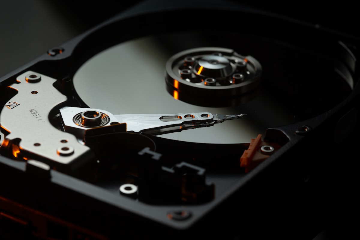
Everything I’ve learned from talking to AI/ML teams about their storage struggles, and why the S3 API is at the center of all of them.
What AI/ML Teams Keep Telling Me
Over the past two years, I’ve talked to dozens of teams building AI infrastructure. Training pipelines, inference platforms, data engineering stacks. Different companies, different scales, different cloud strategies. The complaints are remarkably consistent.
“We spend more on S3 API calls than on the storage itself.” “Our data loader is the bottleneck, not the GPUs.” “We built a whole caching layer just to avoid LIST calls.” “Checkpointing takes so long our GPUs sit idle.” “We tried three different data loading libraries before one worked.”
Every conversation circles back to the same root cause: the S3 API. Not S3’s throughput (that’s fine). Not S3’s durability (that’s excellent). The API itself. The operations it exposes, the operations it doesn’t, and the workarounds that every team independently reinvents.
This post is the long version of what I tell those teams. The S3 API is the POSIX of cloud storage. Its limitations are now the ceiling for innovation. And every workaround the industry has built on top of it is an admission that the foundation is cracked.
The Accidental Standard
In March 2006, Amazon launched S3 with five operations: PUT, GET, DELETE, HEAD, and LIST. The namespace was flat. The consistency model was eventual. The interface was HTTP. The pricing was pay-per-request.
It was, by any engineering measure, primitive. No append. No partial update. No transactions. No server-side compute. No streaming. Error responses in XML. A list operation that returns at most 1,000 keys per page, with no server-side filtering, no sorting beyond lexicographic, and no metadata projection.
Twenty years later, S3 is the most widely implemented storage API in computing history. Every cloud provider speaks it. Every analytics engine queries through it (Spark, Trino, DuckDB, Flink, Athena, Redshift, BigQuery). Every table format builds on it (Iceberg, Delta Lake, Hudi). Every ML framework reads from it (PyTorch, TensorFlow, Hugging Face, NVIDIA DALI). Every object storage system implements it (MinIO, Ceph RGW, Cloudflare R2, Backblaze B2, Wasabi, DigitalOcean Spaces). Kubernetes has COSI (Container Object Storage Interface) as the native standard for provisioning S3-compatible buckets.
The S3 API won. And now it’s in the way.
The Seven Limitations That Matter
1. No Append
S3 has no append operation. Every write is a full object replacement. If you’re ingesting a streaming log, a growing CSV, or a checkpoint file that accumulates data over time, your only option is multipart upload. That requires a minimum of N+2 requests (InitiateMultipartUpload, N UploadPart calls, CompleteMultipartUpload), enforces a 5 MiB minimum part size, and demands an XML request body for completion.
If a multipart upload is never completed or aborted, the uploaded parts remain in storage indefinitely, silently accumulating charges. AWS’s own documentation recommends configuring lifecycle rules with AbortIncompleteMultipartUpload to auto-clean. That’s an admission that the protocol’s failure mode is silent data accumulation. Storage Lens exists partly to discover accounts hemorrhaging money from orphaned uploads.
The 100 GB file uploaded as 800 x 128 MB parts? On AWS, that’s 802 billable requests. On-prem S3-compatible systems like MinIO don’t charge per-request, but the protocol overhead is the same: 802 round trips, 802 HTTP transactions, and an XML completion body. The streaming ingest that writes 1 KB every second? That’s either one multipart upload held open for hours (with timeout risks) or thousands of tiny objects that must be compacted later.
AWS eventually added append operations, but only in S3 Express One Zone directory buckets, via the x-amz-write-offset-bytes header. Standard S3 buckets, where 99% of data lives, still cannot append. Azure Blob Storage has had Append Blobs since inception. The absence in S3 is not a technical limitation. It’s an API limitation that has calcified into an ecosystem constraint.
2. No Partial Update
S3 supports byte-range GET (the Range header for downloads works fine). But there is no byte-range PUT. No PATCH. No partial update of any kind.
To modify one byte of a 10 GB object, you re-upload 10 GB.
This makes S3 fundamentally unsuitable as a mutable data store without application-level chunking. Every system that needs in-place updates (databases, append-optimized logs, memory-mapped files) must either avoid S3 or build an entire abstraction layer on top of it. Azure Blob Storage has Page Blobs with random read/write on 512-byte-aligned pages. S3 has nothing.
The workaround is to shard your data into small objects and manage them yourself. This is exactly what every lakehouse table format does: Iceberg, Delta Lake, and Hudi decompose tables into immutable Parquet files and manage them through metadata. It works. But the architectural complexity of every table format is, in part, compensation for a missing primitive in the storage API.
3. LIST Is a Full Table Scan
ListObjectsV2 returns at most 1,000 keys per page. Listing 1 million keys requires a minimum of 1,000 API calls, each returning a paginated XML response with continuation tokens. There is no server-side filtering beyond prefix matching. No filtering by metadata, size, last-modified date, or tags. No sorting other than lexicographic. No projection. You get every field for every key whether you need it or not.
At scale, this becomes pathological. Joshua Robinson documented listing 67 billion objects in a single bucket. That required millions of LIST calls and careful parallelization across prefix ranges. S3’s 5,500 GET/HEAD requests per second per partitioned prefix means a naive listing of that bucket would take days.
Every analytics query that begins with “find me the Parquet files matching this partition” starts with LIST calls. Every garbage collection sweep that identifies orphaned objects starts with LIST calls. Every data governance audit that inventories a bucket starts with LIST calls. And every one of those LIST calls is O(n) in the number of keys, paginates at 1,000, and cannot be filtered server-side.
GCS does this marginally better. Its JSON API returns only requested fields (projection), reducing payload size. But the fundamental problem is the same: flat-namespace listing is an inherently expensive operation that the API provides no tools to optimize.
4. No Server-Side Compute
Every byte stored in S3 must traverse the network to be processed. There is no way to push computation to the data.
AWS tried twice to fix this. Both attempts failed.
S3 Select (2017-2024) pushed SQL queries down to S3 for CSV, JSON, and Parquet. It supported a limited SQL subset with no JOINs, no subqueries, no aggregation beyond basic functions. For Parquet files, which already have column pruning and predicate pushdown at the format level, S3 Select offered minimal improvement. AWS deprecated S3 Select to new customers in July 2024, recommending Athena or client-side filtering as replacements.
S3 Object Lambda (2021-2025) invoked Lambda functions to transform objects on read. On-the-fly redaction, format conversion, enrichment. Lambda cold-start latency added 100ms-1s+ per request. Per-invocation cost stacked on top of S3 pricing. Execution was capped at 60 seconds. Adoption was low enough that AWS restricted it to existing customers in November 2025.
The lesson: server-side compute in object storage is hard. Both attempts were deprecated within five years of launch. The compute belongs in purpose-built query engines (Athena, Spark, Trino), not in the storage layer. But this means every byte of data must leave the storage system before any processing can happen, and that inefficiency grows linearly with data volume.
5. XML in 2026
S3 error responses are XML. CompleteMultipartUpload request bodies are XML. ListBuckets, ListObjectsV2, and ACL responses are XML. CopyObjectResult is XML. DeleteObjects (multi-object delete) request bodies are XML.
Every S3 client in 2026 must parse and generate XML for core operations. Every SDK carries XML serialization dependencies. Every error handler must extract structured information from XML payloads. Every CompleteMultipartUpload call must construct an XML body listing part numbers and ETags, and a malformed XML body is a common failure mode documented across multiple SDK issue trackers.
The industry moved to JSON a decade ago. GCS has a full JSON API. Azure Blob Storage uses JSON. Every modern REST API uses JSON. S3 cannot change because every existing client depends on XML responses, and changing the wire format would break the entire ecosystem.
This is the compatibility trap in miniature: a design decision from 2006 that wasn’t wrong at the time, but cannot be corrected in 2026 without fracturing the installed base.
6. No Real-Time Change Streams
S3 Event Notifications are asynchronous, delivered via SNS, SQS, Lambda, or EventBridge. AWS documentation states they are “typically delivered in seconds but can sometimes take a minute or longer.” Delivery is at-least-once, with no exactly-once guarantee. There is no WebSocket, gRPC stream, or Server-Sent Events interface for watching bucket changes in real time.
For systems that need to react immediately to new data (real-time ETL, streaming analytics, cache invalidation, event-driven architectures) S3 notifications are too slow, too unreliable, and too loosely coupled. The workaround is polling: periodically LIST the bucket and diff against the previous state. On AWS, every poll is a billable LIST call. On-prem you skip the bill, but you still pay in latency, wasted bandwidth, and CPU cycles. Most polls find nothing new.
Azure Blob Storage has Change Feed with append-only log semantics. GCS has Pub/Sub notifications with stronger delivery guarantees. S3’s event model was designed for batch-oriented workflows where minutes of delay are acceptable. For real-time data pipelines, it’s insufficient.
7. No Multi-Object Transactions
There is no way to atomically update multiple objects in S3. You cannot say “put these three objects or none of them.” You cannot say “delete this object only if that object exists.” You cannot implement a consistent two-phase commit across objects.
Before August 2024, even single-object conditional writes were impossible natively. The workaround for multi-writer coordination was DynamoDB-based locking (which is how Delta Lake manages multi-cluster writes on S3), external coordination services (ZooKeeper, etcd, Consul), or write-ahead logging patterns that add latency and complexity.
AWS added conditional writes in August 2024 with If-None-Match for write-once semantics and If-Match for compare-and-swap via ETag. This is single-object CAS only. Multi-object atomicity remains impossible. If your application needs to update a metadata index and a data file atomically (which is what every table format does on every commit) you must build your own coordination on top of an API that provides none.
Project Nessie addresses this with git-like semantics (branches, commits, multi-table atomic commits) layered on top of object storage. But Nessie is infrastructure you must deploy, manage, and scale. Infrastructure that exists because the storage API lacks a primitive.
What ML Actually Needs (And What S3 Can’t Provide)
The mismatch between S3 and modern workloads is most acute in machine learning, where data access patterns diverge completely from what S3 was designed for.
The Shuffle Problem
PyTorch’s DataLoader assumes random access to individual samples. On S3, this is catastrophic: each random read is a separate GET request with 10-100ms latency. A training run that reads 10 million samples per epoch means 10 million GET requests. On AWS, that’s $4 per epoch in request costs alone. On-prem S3 systems dodge the per-request bill, but the latency problem is identical: 10 million sequential HTTP round trips is slow no matter who runs the servers.
The entire ML data loading ecosystem exists to work around this:
- WebDataset packs training samples into POSIX tar archives (100 MB-1 GB shards), converting random access into sequential I/O. Shuffles at shard level, then within a buffer. Reports 3-10x throughput improvement over per-sample access.
- MosaicML StreamingDataset (Databricks) was built after the team “tried for weeks to get existing solutions like TorchData or WebDataset to work.” It’s a drop-in IterableDataset replacement with deterministic resumption across preempted training runs.
- FFCV uses a custom
.betonformat with internal sharding for higher-quality randomness than shard-level shuffle. - Hugging Face datasets streams from Arrow-format files with configurable shuffle buffers, and in testing, generated over 100,000 S3 requests in under a minute, causing IP-level throttling.
Every one of these libraries is an application-layer workaround for the fact that S3 has no concept of “iterate over this dataset in shuffled order” or “prefetch the next N samples.”
The Fan-Out Problem
Data-parallel training means 1,000 GPUs reading the same dataset. If each GPU fetches its own copy from S3, you get 1,000x request amplification. S3’s per-prefix rate limit of 5,500 GET/s means 1,000 workers targeting the same prefix will be throttled immediately.
WebDataset’s solution is to split shards across workers (20 tar files across 2 GPUs via nodesplitter). MosaicML Streaming notes that downloading ImageNet from AWS S3 costs ~$3 per machine. At 4 machines, that’s $12, and it scales linearly. On-prem S3 avoids the dollar cost, but the request amplification is the same: 1,000 workers hitting the same prefix will saturate your cluster’s metadata handling regardless of pricing model.
The Checkpoint Problem
Model checkpoints must be written quickly (to minimize GPU idle time) and atomically (a half-written checkpoint is worse than no checkpoint). Checkpoint sizes range from gigabytes to hundreds of gigabytes. NVIDIA’s DGX SuperPOD reference architecture specifies 40-125 GB/s aggregate write bandwidth for checkpointing.
S3’s inconsistent latency (p99 write latency exceeding 100ms) makes it poorly suited for time-critical checkpoint writes. A 100 GB checkpoint to S3 at ~1 GB/s takes 100 seconds. That’s 100 seconds of GPUs sitting idle, which at $3/GPU-hour across 1,000 GPUs costs $83 per checkpoint pause.
This is exactly why DeepSeek built 3FS. A purpose-built distributed filesystem with RDMA, CRAQ-based consistency, and 7.3 TB/s aggregate read throughput. Not because they wanted to build a filesystem, but because S3’s per-request latency model and lack of POSIX random-access semantics couldn’t meet their checkpoint write and data shuffling requirements. (To be clear: the S3 protocol doesn’t limit aggregate throughput. MinIO’s AIStor has demonstrated 20+ TiB/s at line rate over S3. The problem is access pattern, not bandwidth.)
The KV Cache Problem
LLM inference KV cache uses paged attention with 16-64 KB pages. These small, non-contiguous chunks require sub-millisecond latency for offload and reload. S3’s 10-100ms latency is three orders of magnitude too slow. The result: a parallel ecosystem of KV cache solutions (LMCache, Mooncake, InfiniStore, NVIDIA’s BlueField-4-powered CMX) that exists entirely because the object storage API cannot serve small objects fast enough.
S3 was designed for web applications uploading images and serving static files. ML workloads need shuffle-and-stream, high fan-out, atomic checkpoints, and sub-millisecond KV access. The gap is not a tuning problem. It’s a fundamental API mismatch.
The Compatibility Trap
The S3 API cannot be fixed because fixing it would break everything that depends on it. And everything depends on it.
The Ecosystem Is the Moat
MinIO built a $1.47 billion market (projected to $7.13 billion by 2033) on one proposition: full S3 compatibility, on any hardware, at any scale. Cloudflare R2’s pitch: S3-compatible, zero egress fees. Backblaze B2: S3-compatible, cheapest per GB. Tigris: S3-compatible, globally distributed. Every competitor’s first feature is “we speak S3.”
The tools are even more locked in. Apache Spark’s S3AFileSystem is the most-used cloud storage connector in the Hadoop ecosystem. Iceberg’s S3FileIO is the default for AWS deployments. Delta Lake’s S3 integration required building an entire DynamoDB-based coordination layer for multi-cluster writes. Not because DynamoDB is a good locking primitive, but because S3 doesn’t have one.
When AWS added default data integrity protections to their S3 SDKs in 2025, the change inadvertently made the default SDK settings incompatible with most third-party S3-compatible services, including GCS’s S3 compatibility layer. A non-breaking server change in the SDK broke the ecosystem. That’s how fragile the compatibility surface is.
The LCD Effect
Any feature that enters the S3 API must work on AWS S3, MinIO, GCS (XML API), Azure (S3 compatibility layer), Ceph RGW, Cloudflare R2, and dozens of smaller implementations. This means:
- Conditional writes (August 2024): Every S3-compatible implementation must add
If-Match/If-None-Matchsupport or lose compatibility. - S3 Express One Zone append: Only works on AWS directory buckets. No other provider can implement it without the directory bucket abstraction.
- S3 Tables: AWS-managed Iceberg. Incompatible concept for other providers.
- S3 Vectors: AWS-only. No S3-compatible equivalent exists.
AWS is increasingly shipping features that are S3 in name only. The S3 API is simultaneously too frozen to fix its core problems (XML responses, no append, no byte-range writes) and too AWS-specific to standardize its new capabilities (Express One Zone, Tables, Vectors). The lowest common denominator stays low, and innovation happens outside the API.
The Cost of Chatty Protocols
On AWS, the S3 API’s per-request pricing model creates perverse incentives. Databricks documented streaming workloads generating 17.28 million S3 API calls per day per pipeline at a 500ms trigger interval. That’s $38.71/day, $1,161/month per pipeline. Ten pipelines: $10,000+/month in API costs, not storage costs.
On-prem S3-compatible systems eliminate the per-request charges, but the chattiness of the protocol remains a problem. 17.28 million API calls per day is 17.28 million HTTP round trips, 17.28 million request parsings, and 17.28 million response serializations. That’s CPU and network overhead regardless of whether anyone sends you an invoice.
High-frequency writes produce many small files (the “small file problem”), which degrade query performance and amplify downstream LIST and GET calls. The S3 API has no batched write operation (PUT 100 objects in one request), no coalesce operation (merge these 50 objects into one), and no server-side compaction. Every workaround (compaction jobs, intermediate buffering, write batching) is application-level complexity born from API-level deficiency.
What GCS and Azure Got Right
If we could redesign S3, what would we steal from the competition?
From GCS
- JSON API with field projection. Request only the fields you need. A LIST call that needs only key names and sizes doesn’t return ETags, storage class, owner, and ACL for every object.
- gRPC transport. Google Cloud Storage offers a native gRPC interface alongside REST. 2025 benchmarks show gRPC delivering 107% higher throughput for small payloads, 48% lower latency, 19% lower CPU usage, 34% less memory, and 41% less network bandwidth compared to REST.
- Compose operations. Server-side concatenation of up to 32 objects without downloading and re-uploading. Enables parallel composite uploads and append patterns without multipart upload complexity.
- Resumable uploads. Built-in resumability with session URIs. Failed uploads resume from the last successful byte, not the last successful part.
From Azure
- Append Blobs. A purpose-built blob type optimized for append operations. Logging, streaming ingest, and audit trails work naturally without multipart upload gymnastics.
- Page Blobs. Random read/write on 512-byte-aligned pages. Databases can use blob storage without decomposing every operation into full-object replacement.
- Lease mechanism. Pessimistic concurrency control with 15-60 second exclusive locks. Not elegant, but functional for coordination scenarios where optimistic CAS is insufficient.
- Batch operations. Up to 256 sub-requests per batch call. S3’s
DeleteObjectssupports batch deletes (up to 1,000 keys), but there is no general-purpose batch API for mixed operations.
Neither GCS nor Azure solved every problem. But both shipped primitives (append, partial update, batch, field projection, server-side compose) that S3 lacks in 2026. The S3 API’s missing primitives aren’t unsolved problems. They’re solved problems that S3 chose not to adopt.
The Attempts to Escape
The industry has tried multiple times to move beyond S3. Each attempt reveals something about why it’s so hard.
SNIA CDMI: The Standard Nobody Implemented
The Cloud Data Management Interface (CDMI) was an ISO/IEC standard (17826:2012, updated 2016) that defined a REST-based API for cloud data with rich metadata, capability discovery, and data management. It was thoughtfully designed, thoroughly specified, and comprehensively ignored.
The failure was simple: AWS never implemented it. Without AWS, no ecosystem formed. Without an ecosystem, no tools adopted it. Without tools, no users demanded it. CDMI is now working on version 3.0 with MCP (Model Context Protocol) support for AI. A standard searching for relevance fifteen years after its creation.
A better standard cannot displace a worse standard that has network effects. The S3 API didn’t win because it’s good. It won because it was first, and because everything else was built on top of it.
Iceberg REST Catalog: The Quiet Successor
The most successful “beyond S3” API isn’t a storage API at all. It’s a table catalog API. The Apache Iceberg REST Catalog specification defines a standardized way to discover tables, manage schemas, perform commits, and handle multi-table operations. AWS Glue supports it. Project Nessie implements it. Polaris, Tabular (acquired by Databricks in June 2024), and multiple other catalogs expose it.
The Iceberg REST Catalog works on top of S3, not instead of it. Objects are still stored via the S3 API. But the table-level operations (the operations that actually matter for analytics) happen through a higher-level API that provides what S3 cannot: schema awareness, atomic commits, and multi-object coordination.
This is pragmatic and revealing. The industry didn’t try to fix S3 for structured data. It built a new API layer above S3 for the operations S3 can’t handle, and left S3 to do what it does adequately: store and retrieve blobs.
LakeFS: Git for Data
LakeFS layers git-like operations (branch, commit, merge, revert) on top of object storage. It solves the multi-object atomicity problem that S3 lacks. A commit in LakeFS is an atomic snapshot of the entire repository. Triple-digit user adoption growth, organizations including NASA, Arm, and Volvo, $43M in funding, and the acquisition of the DVC project in November 2025 suggest genuine market demand.
LakeFS exists because S3 has no concept of a consistent snapshot across multiple objects. Every organization that deploys LakeFS is paying the operational cost of running a separate service to compensate for a missing S3 primitive.
Hugging Face Hub: Purpose-Built for ML
Hugging Face took a different approach: forget S3 compatibility, design for ML artifacts. Their Hub API handles model weights, datasets, tokenizers, and configs with purpose-built semantics. In August 2024, they acquired XetHub and replaced Git LFS with a Xet storage backend featuring chunk-level deduplication. This addresses the “upload 70 GB of model weights that differ by 2% from the previous version” problem that S3’s full-object-replacement model handles terribly.
By May 2025, Xet-enabled repositories became the default. Hugging Face then launched “Buckets,” S3-like object storage powered by the Xet backend with content-addressable deduplication. They started by escaping S3, and are now building their own object storage with the primitives that ML actually needs.
DeepSeek 3FS: Escape Velocity
The most dramatic escape from S3 is DeepSeek’s 3FS, open-sourced in February 2025. A distributed filesystem purpose-built for AI training and inference, delivering 7.3 TB/s aggregate read throughput across their production clusters. It uses RDMA, CRAQ for strong consistency, and a FUSE interface. They explicitly chose POSIX semantics over S3 semantics because training frameworks need random access, not object-level GET/PUT.
3FS sorted 110.5 TiB across 8,192 partitions in 30 minutes (3.66 TiB/min). This is the performance profile that ML training demands, and it’s several orders of magnitude beyond what any S3-compatible system delivers.
DeepSeek didn’t build 3FS because they enjoy building filesystems. They built it because their workload demanded sub-millisecond random reads, RDMA transport, and POSIX semantics that the S3 API doesn’t expose. Regardless of how much aggregate throughput the underlying system can deliver.
What AWS Is Actually Doing
AWS isn’t fixing S3. They’re building specialized sub-APIs within S3’s namespace.
S3 Tables (December 2024): Managed Apache Iceberg with 3x faster query throughput and 10x higher TPS than self-managed tables. Automatic compaction, snapshot management, schema evolution. A new “table bucket” type that acknowledges raw object storage isn’t enough for analytics.
S3 Vectors (GA December 2025): Native vector storage for RAG and agents. 2 billion vectors per index, 20 trillion vectors per bucket, ~100ms query latency, up to 90% cost reduction versus purpose-built vector databases. A new data type that acknowledges objects aren’t the only storage primitive AI needs.
S3 Express One Zone (November 2023, price cuts April 2025): Single-digit millisecond latency, ~9 GB/s throughput, append operations. A new storage class that acknowledges S3 Standard’s latency profile is too slow for hot data paths. But single-AZ only, 8x the storage cost, and requires a different bucket type with different API behavior (LIST doesn’t return lexicographic order).
Conditional writes (August 2024): If-None-Match and If-Match for single-object CAS. A primitive that should have existed from day one, arriving 18 years late.
The pattern is clear: AWS is not going to ship “S3 v2.” They’re going to keep the base S3 API frozen (XML, no append, no partial update, no transactions, no streaming) and build increasingly sophisticated features on top of it. Each with its own bucket type, its own pricing model, its own regional availability, and its own compatibility limitations. S3 Tables isn’t S3. S3 Vectors isn’t S3. S3 Express isn’t S3. They’re new products wearing S3’s name.
Jack Vanlightly’s assessment of S3 Express captures the broader dynamic: “The right technology, at the right time, with the wrong price.” The same could be said of S3 itself in 2026: the right ecosystem, at the right scale, with the wrong API.
Credit Where It’s Due: MinIO Saw This Coming
If AWS is addressing S3’s limitations from the cloud side, MinIO is addressing them from the infrastructure side. And in several cases, they got there first.
The MinIO team has consistently been 12-18 months ahead of legacy storage vendors in recognizing that object storage must evolve beyond the bare S3 API. While Dell, NetApp, and Pure Storage were still selling block and file appliances with S3 gateways bolted on, MinIO was shipping native capabilities that address the limitations outlined in this post:
AIStor Tables (GA February 2026): Native Apache Iceberg V3 with the full Iceberg REST Catalog API embedded directly in the object store. No external Hive Metastore. No AWS Glue dependency. No separate catalog service to deploy and manage. Tables and objects coexist in a single system. MinIO shipped this on-premises, on any hardware, without AWS lock-in.
S3 Select replacement: When AWS deprecated S3 Select in July 2024, MinIO kept their implementation alive and extended it. They recognized that server-side query pushdown is genuinely useful for reducing data movement, even if AWS’s implementation was too limited to sustain.
PromptObject: MinIO’s approach to AI-native object access. Structuring and serving objects in formats optimized for LLM consumption and RAG pipelines. While Hugging Face built a purpose-built Hub API and AWS shipped S3 Vectors, MinIO is building similar capabilities within the S3-compatible ecosystem, giving organizations a private, on-premises alternative to Hugging Face Hub for model artifacts and training data.
Line-rate performance: MinIO’s AIStor has demonstrated 20+ TiB/s aggregate throughput over the standard S3 API. This proves that the protocol itself is not the bandwidth bottleneck. When we say S3’s limitations are in access patterns and missing primitives, MinIO is the proof: their implementation maxes out the network while staying within S3 wire compatibility.
The contrast with legacy storage vendors is stark. EMC (now Dell) spent a decade trying to make HDFS work on Isilon. NetApp bolted an S3 gateway onto ONTAP. Pure Storage added S3 to FlashBlade as an afterthought. These companies are adding S3 compatibility to products designed for file and block. MinIO built for S3 from day one, and is now extending beyond it.
MinIO has shifted to a commercial-first model. The AGPL v3 license change came in 2021, the web console was removed from the community edition in early 2025, and in December 2025 the community edition entered maintenance mode. No new features, no accepted PRs, only critical security fixes on a case-by-case basis. The code remains open source under AGPL v3, but the development focus is entirely on AIStor, MinIO’s commercial product. New features (Tables, PromptObject, enterprise management) ship exclusively in AIStor.
That said, their architectural instincts have been right at every turn: S3-native, not S3-bolted-on. Tables, not just objects. AI-aware, not byte-agnostic. The rest of the industry is catching up to positions MinIO staked out years ago. The gap MinIO leaves in the open-source world (a truly community-driven, S3-native object store with native Iceberg, ML-aware data access, and beyond-S3 primitives) is real, and it’s growing.
What the Next Storage API Actually Needs
If you were designing an object storage API from scratch in 2026, freed from backward compatibility, what would it look like?
1. Append and Partial Update as First-Class Operations
APPEND /key with an offset check. PATCH /key with byte-range specification. These are not exotic features. They’re solved problems in Azure Blob Storage, in every database, in every filesystem. Their absence from S3 forces every streaming, logging, and incremental-update workload to build workarounds.
2. Batch Operations
PUT_BATCH [{key1, data1}, {key2, data2}, ...] with atomic semantics: all succeed or none do. This eliminates the need for external coordination services (DynamoDB, ZooKeeper, etcd) for every multi-object write. Table format commits become a single API call instead of a multi-step protocol.
3. Server-Side Filtering and Projection
LIST /prefix?filter=size>1MB&fields=key,size&sort=last_modified&limit=100. The storage system has all the information to evaluate this server-side. Forcing clients to page through thousands of XML responses and filter locally is a waste of network bandwidth, client CPU, and API request budget.
4. Change Streams
WATCH /prefix with a persistent connection (WebSocket, gRPC stream, SSE) that delivers object mutations in order. Real-time ETL, cache invalidation, and event-driven architectures should not require polling.
5. Conditional Multi-Object Writes
PUT_IF [{key1, data1, if_match: etag1}, {key2, data2, if_none_match: *}]. A single request that atomically applies multiple conditional writes. If any condition fails, none apply. Transactional semantics for object storage without requiring a full ACID database.
6. JSON Wire Format
Error responses, list responses, and request bodies in JSON. Optional content negotiation for backward compatibility. XML as a legacy format, not the default.
7. gRPC Transport
An optional gRPC interface alongside REST. GCS demonstrated that gRPC delivers 2x throughput and 48% lower latency for small payloads. For high-throughput data pipelines, the HTTP parsing overhead is measurable.
8. Prefetch and Hint APIs
PREFETCH /prefix/shard-{00..99}.tar. Tell the storage system what you’ll need next. HINT /key priority=high. Inform caching and placement decisions. ML training pipelines have deterministic access patterns (epoch-based iteration over a fixed dataset). The storage system should exploit this predictability.
The Pragmatic Path
None of this means you should stop using S3. The ecosystem is real. The tooling is mature. The compatibility is valuable. Abandoning S3 compatibility would be architectural malpractice for any storage system that wants adoption.
The pragmatic path is what AWS is doing, but open:
S3-compatible base layer. Full S3 API support (XML and all) so that every existing tool works without modification. Spark reads from it. Iceberg writes to it. PyTorch loads from it. The investment that the ecosystem has made in S3 integration is real and must be honored.
Extended API for what S3 can’t do. Batch operations, change streams, append, server-side filtering, gRPC transport. Exposed through additional endpoints that don’t break S3 compatibility but provide escape hatches for workloads that need them.
Native ML data access. Epoch-based iteration, shuffle-and-stream, prefetch hints, fan-out delivery. The patterns that WebDataset, MosaicML Streaming, and FFCV implement in application code should be storage-system primitives. A POST /bucket?batch-get that returns a TAR stream of objects in shuffled order. A POST /bucket?batch-epoch that registers an epoch and delivers objects in deterministic shuffled order across workers.
Table and vector awareness. Iceberg REST Catalog embedded in the storage system, not bolted on. Vector indexes as a native data type. Schema-aware replication and governance. The operations that matter for analytics and AI should not require separate infrastructure.
The API Is the Ceiling
The S3 API’s dominance is both its greatest achievement and the industry’s biggest constraint. It unified an ecosystem. It enabled interoperability at a scale no storage standard has achieved before or since. It made object storage the default for an entire generation of data infrastructure.
But every innovation now happens despite the S3 API, not because of it:
- Table formats exist because S3 has no schema awareness
- LakeFS exists because S3 has no multi-object atomicity
- WebDataset exists because S3 has no shuffle-and-stream
- DeepSeek 3FS exists because S3’s per-request latency and lack of random-access semantics don’t fit ML training’s access patterns
- S3 Express One Zone exists because S3 Standard is too slow
- S3 Tables exists because S3 doesn’t understand Iceberg
- S3 Vectors exists because S3 doesn’t understand embeddings
Each of these is an admission that the S3 API has become the ceiling, not the floor. The question isn’t whether we need something beyond S3. Every system built in the last five years has already answered that. The question is whether the “beyond S3” capabilities will be proprietary AWS features, fragmented open-source workarounds, or native primitives in the next generation of storage systems.
SNIA’s CDMI proved that a better standard can’t displace a worse one through technical merit alone. But Iceberg’s REST Catalog proved that purpose-built APIs can coexist with S3, addressing specific limitations without demanding a wholesale replacement.
The S3 API won the war. The next battle is everything it can’t do.
S3 API documentation from AWS. S3 Select deprecation from AWS Storage Blog. S3 Object Lambda maintenance mode from AWS documentation. S3 Express One Zone analysis from Jack Vanlightly and WarpStream benchmarks. S3 conditional writes from AWS announcement. S3 API cost analysis from Databricksters. GCS gRPC benchmarks from Google Cloud. MosaicML StreamingDataset from Databricks Blog. DeepSeek 3FS from GitHub. 67 billion object listing from Joshua Robinson. MinIO market data from Growth Market Reports. Hugging Face Xet integration from Hugging Face Blog. LakeFS from lakefs.io. SNIA CDMI from snia.org. Iceberg REST Catalog spec from iceberg.apache.org. NVIDIA DGX SuperPOD storage requirements from CudoCompute. S3 latency benchmarks from nixiesearch and Tigris.

A case for Rust (and a reality check on AI-generated binaries).
Part I: Go Was Never Designed for Storage
Go is a phenomenal language for API servers, CLI tools, DevOps infrastructure, and network services. Google built it to solve a specific problem: getting networked services written and deployed quickly with large teams. And it nailed that.
But storage systems aren’t network services with a database behind them. They are the database. They sit at the bottom of the stack, one abstraction layer above raw disk and kernel syscalls. At that layer, the same design choices that make Go productive start working against you.
The Garbage Collector: Your Latency Enemy
Go’s garbage collector is impressive engineering. It’s concurrent, it’s low-pause, and it’s gotten better with every release. But “low-pause” is not “no-pause,” and storage systems care about tail latency at percentiles that web services don’t.
Consider a storage node handling 10,000 concurrent object GETs. Each request allocates:
- A buffer for reading from disk (4 KB to 1 MB)
- A checksum computation context
- HTTP response headers and framing
- Metadata structs loaded from the object index
Under sustained load, this creates millions of small, short-lived allocations per second. The GC must trace and collect all of them. Even with Go 1.22+‘s improved pacer, GC pauses of 0.5-2ms are common under memory pressure. At the p99.9 level, these compound into visible latency spikes.
This is why every serious Go storage system ends up building its own memory management layer on top of Go’s runtime. NVIDIA’s AIStore has memsys, a slab allocator that pre-allocates large chunks and manually manages sub-allocations to reduce GC pressure. CockroachDB built a custom arena allocator. Badger uses mmap to sidestep the GC entirely for its value log.
When you’re building a framework on top of your language’s memory model to avoid using your language’s memory model, that’s the language telling you it wasn’t designed for your workload.
Rust’s answer: No GC. Period. Memory is allocated and freed deterministically via ownership and borrowing. When a buffer goes out of scope, it’s freed immediately. No tracing, no pausing, no surprises. A storage node under identical load has flat, predictable latency because memory reclamation is woven into the control flow, not running as a parallel process competing for CPU time.
goroutines: Convenient, Uncontrollable
Go’s goroutine scheduler is a cooperative, M:N threading model. It’s elegant for request-handling workloads where thousands of goroutines block on network I/O. But storage systems have a different concurrency profile: they mix CPU-bound work (checksumming, erasure coding, compression) with I/O-bound work (disk reads, network transfers), and they need precise control over which cores do what.
Problems that emerge at scale:
-
No CPU pinning. You can set
GOMAXPROCS, but you can’t pin a goroutine to a core. For NUMA-aware storage (where reading from a locally-attached NVMe is 10x faster than crossing a NUMA boundary), this is a dealbreaker. The scheduler freely migrates goroutines across OS threads, destroying cache locality. -
Cooperative scheduling gaps. A goroutine running a tight Reed-Solomon encode loop won’t yield until the next function call or channel operation. If the loop is pure computation over a large buffer, it holds its OS thread hostage, potentially starving I/O-bound goroutines waiting to serve requests.
-
Stack growth overhead. Goroutines start with a small stack (2-8 KB) that grows dynamically via stack copying. For storage paths that recurse through codec, compression, encryption, and I/O chains, repeated stack growth and copying adds measurable overhead that doesn’t exist with fixed-size stacks or async state machines.
Rust’s answer: tokio gives you an async runtime where CPU-bound work can be explicitly offloaded to spawn_blocking pools, I/O tasks run on dedicated reactor threads, and you control thread affinity, pool sizes, and scheduling priorities. You’re not fighting a general-purpose scheduler. You’re configuring one built for your workload.
The Safety Illusion
Go advocates often cite “no unsafe” as a safety advantage. But Go achieves memory safety by hiding low-level operations behind a runtime, not by proving their absence. The result:
- Data races compile fine. Go’s race detector is a runtime tool, not a compile-time guarantee. A storage system with a race condition in its metadata index passes
go buildwithout a whisper and corrupts data silently in production. interface{}/anyis an escape hatch. Type assertions at runtime can panic. In a storage system’s hot path, a panicking type assertion means a crashed node and an interrupted I/O operation.sync.Mutexis advisory. Nothing in the type system prevents you from accessing shared state without holding the lock. You just have to remember. Across a 200-file codebase with 15 contributors, “just remember” is not a strategy.
Rust’s answer: Send, Sync, ownership, and borrowing are compiler-enforced. A data race is a compile error, not a runtime crash. Arc<RwLock<T>> makes locking structural. You literally cannot access the inner T without acquiring the lock. The type system is the audit tool.
cgo: The Performance Cliff
Storage systems frequently need to call into C libraries: liburing for io_uring, ISA-L for SIMD erasure coding, OpenSSL or BoringSSL for encryption. Go’s cgo makes this possible but painful:
- Each cgo call costs ~200ns of overhead (goroutine stack switch to a system thread). For a storage system making millions of small I/O calls per second, this adds up to seconds of overhead per second of wall time.
- cgo defeats escape analysis. Any pointer passed to C is forced to the heap, eliminating stack allocation optimizations that Go relies on for performance.
- cgo binaries are harder to cross-compile and statically link, complicating deployment.
Rust’s answer: FFI is zero-cost. Calling a C function from Rust has the same overhead as calling it from C. No stack switches, no heap escapes, no runtime coordination. And increasingly, pure-Rust implementations (ring, aws-lc-rs, reed-solomon-simd) eliminate the need for C entirely, with equivalent performance thanks to LLVM’s optimizer and explicit SIMD intrinsics.
Part II: The Great Migration, Go to Rust Is Now Feasible
Three years ago, rewriting a Go storage system in Rust was a multi-year, multi-team bet. That’s no longer true.
AI-Assisted Translation Is Real (and Getting Better)
Modern LLMs can translate Go to idiomatic Rust with surprising fidelity. Not line-for-line transliteration, but actual idiomatic translation:
- Go’s
interfacebecomes Rust’strait - Go’s
goroutine + channelbecomes Rust’stokio::spawn + mpsc - Go’s
sync.RWMutexbecomes Rust’sArc<RwLock<T>> - Go’s
errorreturns become Rust’sResult<T, E> - Go’s
deferbecomes Rust’sDroptrait
We’re not talking about toy examples. Teams are using Claude, Copilot, and specialized tools to translate entire packages (HTTP handlers, serialization logic, test suites) and then manually auditing the output for correctness. The audit step is critical, but it reduces a 6-month rewrite to a 6-week effort for a moderately-sized codebase.
The Rust Ecosystem Caught Up
The “Rust doesn’t have libraries” argument died somewhere around 2023:
| Capability | Go | Rust |
|---|---|---|
| HTTP server | net/http, gin, chi | axum, actix-web, hyper |
| Async runtime | goroutines (built-in) | tokio, async-std |
| Serialization | encoding/json, protobuf | serde, bincode, prost |
| Crypto | crypto/*, boring | ring, aws-lc-rs, rustls |
| Object storage SDK | aws-sdk-go | aws-sdk-rust |
| Metrics | prometheus/client_golang | prometheus-client |
| CLI | cobra, pflag | clap |
| Testing | testing (built-in) | cargo test, proptest, criterion |
For every Go library a storage system depends on, there’s a mature Rust equivalent, often with better performance characteristics because it doesn’t carry a runtime.
Incremental Migration Is Possible
You don’t have to rewrite everything at once. The practical path:
-
Start with the data plane. Rewrite the hot path (the code that reads/writes bytes, computes checksums, encodes erasure shards) in Rust. Expose it as a C-compatible library. Call it from Go via cgo. Yes, cgo has overhead, but it’s localized to the boundary, and the Rust code runs at native speed.
-
Migrate the I/O layer. Replace Go’s
os.Fileandio.Readerchains with Rust’stokio::fsandio_uringwrappers. This is where the biggest performance gains live. -
Migrate the server. Replace
net/httpwithaxum+hyper. This is the largest change but also the most mechanical. HTTP handlers are structurally similar across languages. -
Delete the Go. Once all components are in Rust, remove the cgo bridge and ship a single, statically-linked binary with no runtime dependencies.
Part III: No, AI Will Not “Just Generate Binary”
Elon Musk recently predicted that by late 2026, AI will bypass programming languages entirely and generate optimized machine code directly from natural language prompts. As he put it: “Create optimized binary for this particular outcome”. No source code, no compiler, no programming language involved.
He’s wrong, and it’s worth explaining why.
Compilers Already Do This (Deterministically)
The translation from human intent to machine code is a solved problem with 70 years of engineering behind it. LLVM, GCC, and the Rust compiler transform high-level code into optimized machine instructions using:
- Register allocation algorithms with mathematical proofs of optimality
- Instruction scheduling tuned to specific microarchitectures (Zen 4, Sapphire Rapids, Graviton 3)
- Auto-vectorization that maps scalar loops to SIMD instructions
- Link-time optimization across translation units
- Profile-guided optimization from real-world execution traces
An LLM generating binary would need to replicate all of this, not approximately, but exactly, because a single wrong instruction in a storage system’s I/O path means silent data corruption. LLMs are stochastic. Compilers are deterministic. Replacing a deterministic system with a stochastic one is a regression, not progress.
You Cannot Iterate on Binary
Software engineering is 10% writing new code and 90% reading, modifying, debugging, and reviewing existing code. Binary is opaque:
- You can’t diff two binaries meaningfully. Code review is impossible.
- You can’t set a breakpoint in the “intent” that generated the binary. There’s no source map.
- You can’t audit for security vulnerabilities. Was there a buffer overflow in that AI-generated binary? A timing side-channel in the crypto path? Without source code, you’d need to reverse-engineer every output.
- You can’t version-control it. Git stores text diffs efficiently. Binary blobs are opaque, non-mergeable, and storage-expensive.
Platform Portability Doesn’t Exist in Binary
Source code compiles to any target: x86-64, ARM64, RISC-V, WASM. A single Rust crate supports all of them via cargo build --target. An AI generating binary would need to produce separate, verified outputs for every architecture, every operating system, and every ABI version. The combinatorial explosion is precisely why we invented compilers and portable languages in the first place.
What AI Actually Does Well for Code
AI isn’t replacing compilers. It’s replacing boilerplate and translation labor:
- Language migration (Go to Rust, Python to TypeScript). Structurally mechanical work.
- Test generation. Producing property tests and edge cases from function signatures.
- Documentation. Explaining what code does in natural language.
- Code review. Catching common patterns like unchecked errors, missing locks, SQL injection.
- Scaffolding. Generating project structure, CI configs, deployment templates.
These are real productivity gains. A good engineer with AI tools is easily 2-5x more effective than without them. But they work because source code exists. There’s a human-readable, machine-parseable, version-controllable artifact that both humans and AI can reason about.
AI won’t replace compilers. It’ll make engineers faster at writing code in languages like Rust where the compiler has enough information to optimize aggressively.
The Real Disruption
If Musk’s prediction has a kernel of truth, it’s this: the barrier to entry for systems programming is dropping fast. Writing a storage system in Rust in 2023 required deep expertise in ownership, lifetimes, async patterns, and unsafe abstractions. In 2026, an engineer with Go experience and access to AI tools can produce correct, idiomatic Rust, with the AI handling the mechanical translation and the engineer focusing on architecture and correctness.
That’s not the death of programming. It’s the opposite. Systems programming is becoming accessible to a much wider pool of engineers. And that makes Rust more relevant, not less, because it’s the language where the compiler catches your mistakes before they ever hit production.
Conclusion
Go gave us a generation of storage systems that were quick to build and easy to maintain. That was the right call at the time. But data volumes keep growing, latency budgets keep shrinking, and Go’s runtime overhead has become a ceiling that no amount of clever engineering can punch through.
Rust removes that ceiling. With AI-assisted migration cutting the cost from “multi-year rewrite” to “one quarter,” the question isn’t whether to migrate anymore. It’s when.
As for AI generating binary directly: we’ll believe it when we see a storage system handling petabytes of production data from AI-generated machine code with no source, no debugger, and no way to audit what it’s doing. Until then, we’ll keep writing Rust.
References: Elon Musk’s comments on AI-generated binary from his post on X (February 2026). Technical counterarguments draw from Adam Holter’s analysis and decades of compiler engineering literature.
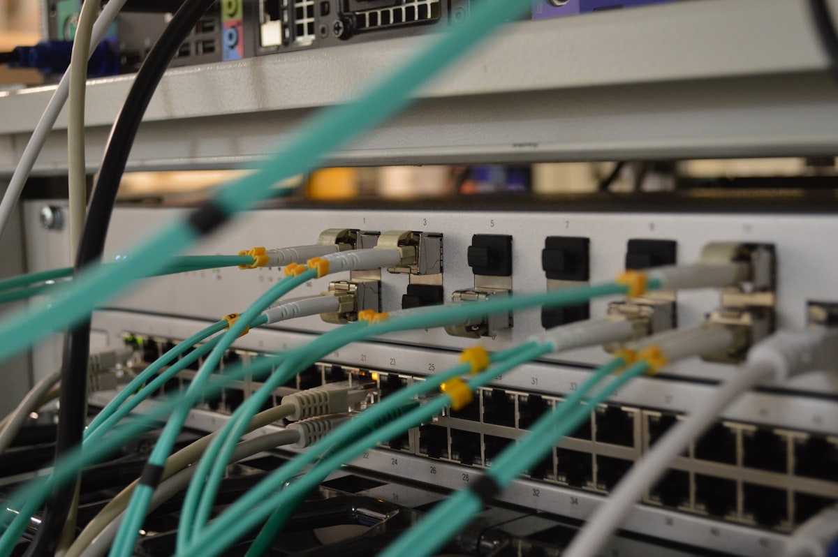
Every storage protocol you need to understand, why it exists, and which ones will survive the next decade.
Updated March 16, 2026: NVIDIA officially rebranded ICMS to CMX (Context Memory Extensions) at GTC 2026. References updated throughout.
Start Here: What Is a “Storage Protocol” Anyway?
Before we get into it, let’s agree on terms. A storage protocol is the language a computer uses to talk to the thing holding its data. It defines how bytes get from Point A (your application) to Point B (a disk, a flash chip, a cloud bucket, a GPU’s memory). Different protocols exist because Point B keeps changing, and so does what we’re asking it to do.
Think of it like ordering food. You can walk into the kitchen and grab it yourself (local storage). You can call a waiter (a network protocol). You can use a delivery app (cloud API). Each method has trade-offs in speed, convenience, and how much control you have over what arrives.
If you just want the punchline (which protocol wins for which AI workload), skip to the cheat sheet near the end. But if you want to understand why, let’s walk through every layer.
Layer 1: Local Storage, the Drives Themselves
Local storage means a physical device plugged directly into your machine. No network, no middleman. Three technologies dominate.
Hard Disk Drives (HDDs)
A spinning metal platter coated in magnetic material, with a tiny arm that floats nanometers above the surface reading and writing data. The same basic design since IBM shipped the first one in 1956 (it was the size of two refrigerators and held 5 MB).
How they work. The arm seeks to a position on the platter, waits for the right sector to spin underneath, and reads or writes magnetically. This mechanical motion is why HDDs have seek times measured in milliseconds. The arm literally has to move.
Speed. Sequential reads around 200-250 MB/s for modern drives. Random I/O is the killer: maybe 100-200 IOPS because each operation requires a physical seek.
Where they still win. Cost per terabyte. An 18TB HDD costs around $250 in early 2026. That’s roughly $0.014/GB. Nothing else comes close for bulk capacity. Cold archives, backup targets, surveillance footage, regulatory retention. Any workload where you need petabytes and can tolerate latency.
AI relevance. HDDs still hold the majority of the world’s training data in cold storage tiers. The dataset you download from Hugging Face probably lived on spinning rust before it reached you.
Solid State Drives (SSDs, SATA)
No moving parts. Data is stored in NAND flash cells: tiny transistors that trap electrons to represent bits. SATA SSDs plug into the same connectors that HDDs use, which made them a drop-in upgrade starting around 2010.
How they work. Flash cells are organized into pages (4-16KB) and blocks (256-512 pages). You can read or write individual pages, but you can only erase an entire block at once. This asymmetry (read a page, erase a block) is the source of most SSD complexity. A chip called the Flash Translation Layer (FTL) manages the mapping.
Speed. SATA tops out at 600 MB/s (the interface is the bottleneck, not the flash). Random IOPS around 50,000-100,000.
AI relevance. Minimal for training workloads. SATA’s 600 MB/s ceiling is a hard wall. But plenty of inference servers still have SATA SSDs for the OS and model weight storage where latency isn’t the primary concern.
NVMe SSDs: The Game Changer
NVMe (Non-Volatile Memory Express) is what happens when you throw away the legacy interface and design a protocol specifically for flash. Instead of talking through the SATA/AHCI stack (designed for spinning disks), NVMe talks directly over PCIe lanes, the same high-speed bus your GPU uses.
How they work. Same NAND flash as SATA SSDs, but the protocol supports 65,535 queues with 65,536 commands each (vs SATA’s single queue of 32 commands). That’s the difference between a single-lane road and a 65,535-lane highway.
Speed (as of early 2026). PCIe Gen4 x4: 7 GB/s reads. Gen5 x4: 14 GB/s. Random IOPS: 1,000,000+. A single NVMe drive is faster than an entire rack of HDDs.
Form factors. M.2 (the little stick in your laptop), U.2 (2.5” enterprise), and the newer EDSFF (ruler-shaped, designed for maximum density: 32 drives in 1U for 4+ PB in less than 2 inches of rack space).
AI relevance. This is where NVMe earns its keep. A single GPU training run might read hundreds of terabytes. NVMe’s bandwidth means a node with 24 drives can deliver 168 GB/s to local applications. That’s enough to feed multiple GPUs without starving them. NVIDIA’s GPUDirect Storage (GDS) can even bypass the CPU entirely. Data flows straight from NVMe to GPU memory over PCIe.
The cost (early 2026). NVMe is 3-5x the price per TB of HDDs. But price-per-IOPS and price-per-GB/s tell a completely different story. For performance-sensitive workloads, NVMe is the cheapest option by far.
Layer 2: Making Remote Storage Feel Local
What if the storage isn’t physically in your server but you want your applications to think it is?
Direct-Attached Storage (DAS)
DAS is technically “remote” in the sense that the drives live in a separate enclosure (a JBOD, Just a Bunch of Disks), connected to your server by a cable. But the connection is direct, not over a network. Common interfaces include SAS (Serial Attached SCSI) cables that can connect 100+ drives to a single server.
Think of it as an extension cord for your storage. Your server sees the drives as if they were internal. No network stack, no shared access. Simple, fast, cheap.
AI use case. DAS JBOFs (Just a Bunch of Flash) are the storage backbone of many GPU training clusters. NVIDIA DGX systems ship with NVMe SSDs as DAS. When you need raw bandwidth without network overhead, DAS wins.
Network-Attached Storage (NAS) and NFS
NAS puts storage on the network and exposes it as a file system. Your server mounts a remote share and accesses files with standard read/write/open/close operations, the same POSIX semantics as a local filesystem.
The protocol. NFS (Network File System), invented by Sun Microsystems in 1984, is the Unix standard. SMB/CIFS is the Windows equivalent. NFSv4.1+ adds parallel NFS (pNFS) for distributing data across multiple servers.
How it feels. You mount -t nfs server:/export /mnt/data and then ls /mnt/data like it’s local. Applications don’t know the difference. That’s the magic, and the trap.
The trap. POSIX file semantics (locks, permissions, open-close-delete atomicity) are expensive to maintain over a network. Every stat() call, every directory listing, every lock check crosses the network. At scale, metadata operations become the bottleneck, not data transfer.
AI relevance. NFS is the most common protocol for AI training data today. Why? Because PyTorch’s DataLoader, TensorFlow’s tf.data, and every ML framework expect a filesystem path. dataset = ImageFolder("/mnt/training-data/") just works. No special SDK, no API calls, no code changes. This simplicity is NFS’s superpower.
Here’s the dirty secret: NFS is often not the right protocol for AI workloads. Training data is read sequentially, shuffled, and never modified. POSIX semantics (locks, permissions, mtime tracking) are pure overhead. But NFS persists because changing the data loading code is friction, and engineers optimize for “works today” over “optimal tomorrow.”
Layer 3: Block Storage, the SAN Era
What Is Block Storage?
Block storage strips away the file abstraction entirely. No filenames, no directories, no permissions. Just numbered blocks (typically 512 bytes or 4KB) on a logical volume. The server sees a raw disk and puts its own filesystem on top.
Think of it as renting an empty apartment. The building (SAN) provides the space, but you bring your own furniture (filesystem) and organize it however you want.
The Rise of the SAN
Storage Area Networks emerged in the late 1990s when databases outgrew local storage. The pitch was simple: build a dedicated high-speed network just for storage traffic, separate from the regular Ethernet LAN.
The protocols:
-
Fibre Channel (FC). The original SAN protocol. Dedicated switches, dedicated cables (fiber optic), dedicated HBAs (Host Bus Adapters). Blazing fast for its era (1 Gb/s in 1997, 64 Gb/s today). Extremely reliable. Extremely expensive. Think of FC like a private highway: fast and uncongested, but you have to build the entire road yourself.
-
iSCSI. “Let’s run SCSI commands over regular Ethernet.” Launched in 2003, iSCSI democratized SANs. Instead of dedicated FC infrastructure, you use your existing network. Slower than FC (Ethernet has more overhead), but dramatically cheaper. The Honda Civic to FC’s Ferrari.
-
Fibre Channel over Ethernet (FCoE). An attempt to get FC’s performance on Ethernet’s infrastructure. Required special “lossless” Ethernet switches. Never gained traction. It combined the complexity of both protocols with the advantages of neither.
A Brief History of SAN Drama
The SAN era (roughly 2000-2015) was the golden age of enterprise storage vendors. EMC (now Dell EMC), NetApp, IBM, Hitachi, Pure Storage built empires selling arrays that cost more than sports cars. What made SANs dominant was databases. Oracle, SQL Server, DB2 all needed consistent, low-latency block I/O with enterprise features like snapshots, replication, and deduplication. Try doing that with a pile of local disks.
The decline. AWS EBS (Elastic Block Store) is essentially a cloud SAN, but you don’t buy the hardware, configure the switches, or hire the SAN admin. On-premises SANs still exist (banks, hospitals, government), but new deployments are increasingly cloud-based or software-defined.
AI relevance. Block storage is critical for databases that support AI workflows: PostgreSQL for metadata, vector databases like pgvector, ML experiment tracking. But you don’t train models on block storage. The block interface (read block 47,382 from LUN 3) is a terrible match for “stream 50TB of images sequentially.”
Layer 4: NVMe over Fabrics, the SAN Reborn
NVMe-oF is the modern answer to the SAN. The concept: extend the NVMe protocol over a network, so remote flash drives appear as if they’re locally attached. Microsecond-level remote storage access.
Why NVMe-oF Exists
Local NVMe is fast: 10 microsecond latency. But what if you have 1,000 NVMe drives in a rack and 100 compute nodes that need access? You can’t plug every drive into every server. NVMe-oF extends the NVMe queuing model over a network fabric, preserving the multi-queue architecture that makes NVMe fast.
The Transport Options
| Transport | Latency Added | Infrastructure Required | Reality Check |
|---|---|---|---|
| RDMA (RoCEv2) | ~5-10 us | Lossless Ethernet (PFC/ECN), specialized NICs | Fastest, but fragile. Configuring lossless Ethernet correctly is an art form. Misconfigure one switch and performance craters. |
| InfiniBand | ~2-5 us | Dedicated InfiniBand switches and HCAs | HPC standard, NVIDIA’s home turf. Fast and reliable, but separate network fabric. |
| TCP | ~30-80 us | Standard Ethernet | Easy to deploy, works everywhere. But 30-80us on top of NVMe’s 10us is a 3-8x latency hit. Still way faster than iSCSI. |
The Promise vs. Reality
The promise. “Remote NVMe that feels local.” Disaggregated storage: separate your compute and storage into independent pools that scale independently.
The reality in 2026. NVMe/TCP works and is widely deployed, but “feels local” is a stretch when you 3x the latency. RDMA is genuinely close to local performance, but requires careful network engineering. InfiniBand delivers on the promise, but only within HPC/AI clusters that already run InfiniBand for GPU-to-GPU communication.
AI relevance. This is big. NVIDIA’s entire inference infrastructure assumes NVMe-oF as the transport between storage and compute. BlueField-4 DPUs speak NVMe-oF natively. When Jensen Huang talks about “AI factories,” the storage fabric connecting thousands of GPUs to petabytes of flash is NVMe-oF over InfiniBand or RoCEv2.
Layer 5: Object Storage, the Quiet Revolution
What Object Storage Is
Object storage throws away everything you know about filesystems and block devices. No hierarchy. No directories. No block addresses. Just three things:
- A key (a string, like
training-data/imagenet/n01440764/n01440764_10026.JPEG) - The data (the bytes)
- Metadata (arbitrary key-value pairs describing the object)
You interact with it through HTTP: PUT to store, GET to retrieve, DELETE to remove, LIST to enumerate. That’s essentially the whole API.
The Origin Story
Amazon launched S3 (Simple Storage Service) on March 14, 2006. It was designed for one thing: giving web applications a place to store files without managing servers. Upload a profile photo, serve a static website, store log files. Nobody was thinking about AI.
Why S3 won. Three things that sound boring but changed everything:
- Pay per use. No upfront hardware purchase. Store one byte or one petabyte, pay only for what you use.
- Infinite namespace. No capacity planning. No “disk full” errors. Just keep writing.
- Eleven nines of durability. 99.999999999%. Meaning if you store 10 million objects, you’d statistically lose one every 10,000 years.
The “Slow” Reputation
For its first decade, object storage had a reputation problem: it was slow. And honestly? It was. Early S3 latency was 50-200ms per request. You couldn’t run a database on it. You couldn’t mount it as a filesystem without hideous performance. It was “archive tier,” the place you put data when you didn’t need it anytime soon.
The reasons were architectural: HTTP overhead, eventually consistent reads (until 2020, S3 could return stale data after a write), and the simple fact that it was designed for throughput and durability, not latency.
The Transformation
Everything changed between 2020 and 2025:
-
Strong consistency (2020). S3 became strongly consistent at no extra cost. Read-after-write consistency for all operations. This single change eliminated the #1 objection from serious workloads.
-
S3 Express One Zone (2023). Purpose-built for latency-sensitive workloads. Single-digit millisecond first-byte latency. 10x faster than standard S3.
-
S3 Tables (2024). Native Apache Iceberg support. Object storage that understands tabular data. 3x faster queries, automatic compaction, built-in catalog.
-
S3 Vectors (2025). Native vector embedding storage and nearest-neighbor search. Sub-second queries over 2 billion vectors.
-
Performance at scale. Modern object stores (MinIO, Ceph RGW, and cloud-native ones) can deliver 100+ GB/s aggregate throughput on commodity hardware. That’s enough to feed a rack of GPUs.
Why Object Storage Is the Future
The contrarian take that’s rapidly becoming consensus: object storage will eat everything.
Not because it’s the fastest protocol for every workload. It isn’t. But because it solves the problems that actually matter at scale:
-
Scale without limits. Filesystems break at billions of files (ask anyone who’s run
lson a directory with 10 million entries). Block storage requires LUN management and capacity planning. Object storage scales to trillions of objects by design. Flat namespace, hash-based distribution, no directory tree to maintain. -
Economics. Object storage on commodity hardware costs 1/10th of enterprise SAN storage. Erasure coding gives you 11-nines durability at 1.5x raw capacity (vs. 3x for replication).
-
HTTP is universal. Any language, any platform, any cloud speaks HTTP. No special drivers, no kernel modules, no vendor lock-in (assuming S3-compatible API).
-
Metadata is first-class. Unlike block and file storage, every object carries its own metadata. This is transformative for data management. Search, classify, govern, and lifecycle data based on its properties, not its location in a directory tree.
-
Immutability is natural. Objects are written once and read many times. This aligns perfectly with training datasets, model checkpoints, audit logs, and regulatory archives. No in-place updates means no corruption, no locking, no read-write conflicts.
Layer 6: Data Lakes and Data Lakehouses
The Data Lake
A data lake is a fancy name for “dump everything into object storage and figure out the schema later.” Coined by Pentaho CTO James Dixon around 2010, the idea was to store raw data (structured, semi-structured, unstructured) in its native format on cheap storage (originally HDFS, now mostly S3-compatible object storage).
The appeal. No upfront schema design. No ETL pipeline to transform data before loading. Just dump your CSV files, JSON logs, Parquet tables, images, and videos into buckets. Analyze later with Spark, Presto, or Hive.
The problem. Data lakes became data swamps. Without schema enforcement, governance, or quality checks, organizations ended up with petabytes of data nobody could find, trust, or use. “Schema on read” sounds liberating until you realize nobody documented the schema.
The Data Lakehouse
The lakehouse architecture (Databricks coined the term in 2020) is the fix. It puts a structured table format (Apache Iceberg, Delta Lake, or Apache Hudi) on top of object storage. You get:
- Schema enforcement. Data types, column constraints, NOT NULL rules.
- ACID transactions. Atomic writes across multiple files.
- Time travel. Query data as it existed at any point in the past.
- Partition evolution. Change how data is organized without rewriting it.
- Open format. Parquet files on object storage, readable by any engine.
Why it matters for AI. A lakehouse is where training data lives in production. Your ML pipeline reads from Iceberg tables on object storage, trains a model, writes evaluation metrics back to another table, and stores model artifacts as objects. All in the same system.
The progression looks like this:
Raw data (logs, events, sensors)
        |
        v
Object Storage (S3-compatible, durable, cheap)
        |
        v
Iceberg Table (schema, versioning, ACID)
        |
        v
Feature Engineering (Spark, Flink, DuckDB)
        |
        v
Training Pipeline (PyTorch DataLoader)
        |
        v
Model Artifacts -> back to Object Storage
Everything in this pipeline speaks object storage. The lakehouse doesn’t replace S3. It adds structure on top of it. This is why object storage is the foundation layer that everything else builds on.
The NVIDIA Factor: Why This All Matters for AI
NVIDIA doesn’t build storage. But NVIDIA increasingly dictates what storage looks like through its certification programs, reference architectures, and the sheer gravitational pull of being the center of the AI universe.
The Current State: File and Block Still Rule
Most AI training clusters today still use NFS or Lustre for training data. Not object storage. File protocols.
Why? Three reasons:
-
PyTorch expects a filesystem.
DataLoader(dataset=ImageFolder("/data/train/"))needs a mounted path. Rewriting data loaders to use S3 APIs is possible (via smart libraries) but adds complexity. -
NVIDIA DGX and certification. NVIDIA’s validated designs (DGX SuperPOD, BasePOD) have historically certified file-based storage partners. WEKA, DDN Lustre/EXAScaler, VAST Data, NetApp: all primarily file/NFS vendors. The certification program ensures these systems can keep GPUs fed. If you want the “NVIDIA Certified” badge, you play by NVIDIA’s rules.
-
Random access patterns. Training with random shuffling requires random reads across a dataset. File protocols handle this naturally. Object storage traditionally adds HTTP overhead per request, making small random reads expensive.
The Shift: Object Storage Is Coming
But the tide is turning. NVIDIA’s storage ecosystem is evolving in a significant direction:
Larger datasets demand object scale. When your training set is 100TB, NFS can handle it. When it’s 10PB (common for foundation model training), you need object storage’s scale-out economics. No NFS server handles 10PB gracefully. Object storage distributes it across hundreds of nodes automatically.
Cloud training is object-native. Every major cloud’s AI training service (AWS SageMaker, Google Vertex AI, Azure ML) reads training data from object storage. Cloud-native training pipelines skip NFS entirely.
New protocols bridge the gap. S3-compatible APIs with range reads, batch operations, and prefetch hints are closing the performance gap. Libraries like AIStore, S3 connector for PyTorch, and fsspec abstract the protocol. Your DataLoader code stays the same, but reads come from S3 instead of NFS.
NVIDIA is broadening. The partner ecosystem is expanding beyond file storage. Fast object storage that can deliver sustained high-bandwidth reads to GPU clusters is becoming a validated tier. The writing is on the wall: object storage with performance guarantees will be a first-class citizen in NVIDIA’s reference architectures.
CMX: Context Memory Extensions
This is the part most storage coverage misses entirely.
At CES 2026, NVIDIA announced what was originally called ICMS (Inference Context Memory Storage). At GTC 2026, they officially rebranded it as CMX (Context Memory Extensions). It’s not a product you buy. It’s a new tier in the memory hierarchy, sitting between local NVMe and shared object storage.
Why it exists. Modern AI inference (especially with large language models and AI agents) builds enormous context windows. When a chatbot maintains a 128K-token conversation, that context lives as a KV (key-value) cache in GPU memory. But GPU HBM is precious and limited. When the KV cache overflows HBM, it needs somewhere to spill.
The memory hierarchy for AI inference looks like this:
| Tier | What | Latency | What Lives There |
|---|---|---|---|
| G1 | GPU HBM | Nanoseconds | Active KV cache, model weights |
| G2 | Host RAM | Microseconds | Overflow KV cache, prefill buffers |
| G3 | Local NVMe | ~100 us | Warm context, model weight shards |
| G3.5 (CMX) | Network flash (RDMA) | Low microseconds | Shared KV cache across pods |
| G4 | Object Storage | Milliseconds | Training data, checkpoints, datasets |
The magic is G3.5. Without CMX, if Agent A builds a context on Node 1 and Agent B needs related context on Node 7, it has to be recomputed from scratch. CMX creates a shared flash tier across the pod, powered by BlueField-4 DPUs with 800 Gb/s RDMA connectivity and Spectrum-X Ethernet. NVIDIA DOCA Memos provides the SDK for managing KV cache across compute nodes with hardware-accelerated encryption.
Why should you care? Because CMX defines what the G4 object storage layer needs to be:
-
Fast enough to pre-stage into CMX. If your object store can’t deliver sustained 100+ Gb/s to the CMX tier, it becomes the bottleneck for the entire inference pipeline.
-
Smart enough to know what to pre-stage. The object store that understands inference patterns (which context windows are reused, which model shards are hot, which datasets feed which agents) will outperform one that treats everything as opaque blobs.
-
Integrated with the NVIDIA ecosystem. NVMe-oF transport, GDS support, Dynamo integration. The storage system that speaks NVIDIA’s language will get the certification, the reference architecture inclusion, and ultimately the deployment.
Putting It All Together: Which Protocol for Which AI Workload?
Let’s get practical.
Data Collection and Preparation
Winner: Object Storage
Raw data arrives from everywhere: web scrapes, sensor feeds, user logs, public datasets. You need scale (petabytes), durability (don’t lose it), and cost efficiency (most of it won’t survive filtering). Object storage with lifecycle policies to tier cold data is the obvious choice.
Feature Engineering and ETL
Winner: Data Lakehouse (Object Storage + Iceberg)
Iceberg tables on object storage give you schema enforcement, versioned datasets, time travel for reproducibility, and engine-agnostic access. Run Spark or Flink for ETL, query with DuckDB for exploration, all reading from the same Iceberg tables.
Model Training
Current Winner: NFS/Lustre. Future Winner: Object Storage
Today, NFS wins because of tooling compatibility and random read performance. But as datasets grow beyond what single NFS servers can handle, and as PyTorch’s data loading ecosystem adds first-class S3 support, object storage’s scale-out architecture becomes necessary. The crossover is happening now for datasets above ~500TB.
Model Checkpointing
Winner: Object Storage
Checkpoints are large (multi-GB to TB), written periodically, and need durability. Object storage with versioning is ideal. Write checkpoint v47, keep the last 10 versions, auto-expire older ones. No filesystem to manage.
Inference: Model Serving
Winner: Local NVMe + CMX + Object Storage (tiered)
Hot model weights on local NVMe (G3). Shared context in CMX (G3.5). Model artifacts and full weight sets in object storage (G4). The tiers work together. CMX pre-stages from object storage, local NVMe caches the hottest data.
Inference: KV Cache and Context
Winner: CMX
This is CMX’s reason for existing. Shared, transient, high-bandwidth context that doesn’t need durability but needs to be accessible across pods. Neither NFS nor object storage is designed for this workload.
Vector Search (RAG)
Winner: Object Storage (with native vector support)
Billions of embeddings need scale-out storage, not a single-node vector database. AWS S3 Vectors showed the direction: vectors as a storage primitive, not a separate system.
The Trajectory: Where This Is All Heading
My prediction for the next five years:
NFS and block storage won’t disappear, but they’ll shrink to niche roles. NFS for legacy compatibility and small-scale training. Block for databases. Neither grows.
Object storage becomes the universal foundation. Not because it’s perfect for every workload, but because it’s good enough for most and best for scale, economics, and data management. The performance gap with file/block protocols shrinks every year. When object storage is within 20% of NFS speed but 10x cheaper at 100x the scale, the math doesn’t lie.
Table formats (Iceberg) and vector indexes become standard features of object storage, not separate products. Just as S3 absorbed consistency, it will absorb tabular and vector capabilities. MinIO’s AIStor Tables and AWS S3 Tables/Vectors are the first wave.
CMX creates a new storage category that didn’t exist before: transient, shared, high-bandwidth context memory. It’s not file, block, or object. It’s something new, purpose-built for AI inference, and it will become as fundamental to AI infrastructure as GPUs are to training.
The storage protocol that wins the AI era isn’t the fastest one. It’s the one that understands data (schemas, embeddings, inference patterns, lifecycle) rather than just moving bytes. Object storage, extended with tables and vectors and integrated with CMX, is on that trajectory. Everything else is arguing about I/O latency while the world moves to data semantics.
The bytes still matter. They always will. But the protocol that just moves bytes and nothing else? That’s the one heading for the history books.
NVIDIA CMX (formerly ICMS) details from the NVIDIA CMX page, NVIDIA Technical Blog, and BlueField-4 announcement. NVMe-oF specifications from NVM Express. Apache Iceberg at iceberg.apache.org. S3 API reference at AWS S3 documentation.

A 37-year-old standard is holding storage back.
Where POSIX Came From (and Why It Made Sense)
In 1983, the IEEE authorized a project to standardize the kernel interface across the proliferating zoo of Unix variants: AT&T System V, BSD, Xenix, SunOS, HP-UX, and others. The result, published in 1988 as IEEE Std 1003.1, was named POSIX (Portable Operating System Interface, the name suggested by Richard Stallman). Its goal was elegantly simple: write your program once, compile it on any conforming Unix, and it works.
POSIX’s I/O model reflected the reality of 1988 computing:
- One machine, one filesystem. Storage was a disk attached to the machine your program ran on. Network filesystems (NFS) existed but were slow, unreliable, and optional.
- Files in directories. The hierarchical namespace (
/home/user/data/file.txt) mapped directly to the on-disk structure of the Unix filesystem (UFS, later ext2/3/4, XFS, ZFS). - Open, read, write, close. Stateful file descriptors tracked your position in a file. The kernel maintained per-process state for every open file.
- Strong consistency. A
write()followed by aread()on the same file descriptor returns the data you just wrote. Always. Immediately. No eventual consistency, no stale reads. - Metadata is cheap.
stat(),chmod(),chown(),utimes(). Querying and modifying file metadata costs a few microseconds because the inode is on a local disk, cached in RAM.
For three decades, this model worked. It worked for workstations, for databases, for HPC (where parallel filesystems like Lustre and GPFS extended POSIX semantics across clusters), for web servers, for everything that ran on Unix.
It worked because the fundamental assumption held: storage is local, or close enough to local that the abstraction doesn’t leak.
That assumption is now false. If you want the short version of why, skip to “The Way Forward” at the end. But if you want the full case, here are six reasons POSIX doesn’t hold up at modern scale.
The Six Sins of POSIX at Scale
1. The Metadata Wall
Every POSIX operation begins with metadata. open() traverses the directory tree, resolving each path component through inode lookups. stat() fetches inode attributes. readdir() enumerates directory entries. On a local ext4 filesystem with VFS caching, these operations complete in microseconds.
On a distributed filesystem with billions of files, they don’t.
A metadata server (MDS) in Lustre, CephFS, or HDFS must handle every stat(), every open(), every readdir() from every client. AI training pipelines that scan millions of small image files (ImageNet: 14 million files, average 100 KB) generate millions of metadata operations per minute. The MDS becomes the bottleneck long before the data servers are saturated.
The standard workaround (“pack your small files into tar archives”) is an admission that the filesystem abstraction has failed. When the recommended practice is to work around the interface rather than use it, the interface is wrong.
Object storage has no metadata server. A key like training/imagenet/n01440764/n01440764_10026.JPEG is hashed directly to a storage node. No directory traversal, no inode lookup, no centralized bottleneck. Flat namespaces scale linearly.
2. The Statefulness Tax
POSIX I/O is stateful. open() creates a file descriptor with an implicit seek position. The kernel tracks this state for every open file, across every process, on every node that mounts the filesystem.
In a distributed system with 1,000 clients, each with 100 open files, the filesystem must maintain 100,000 pieces of state and keep them consistent. If a client crashes, the server must detect the failure and clean up its state (file locks, lease renewals, buffered writes). NFS’s statd and lockd daemons exist solely to manage this complexity, and they are notoriously unreliable.
Object storage is stateless. PUT /key writes an object. GET /key reads it. No open, no close, no seek position, no file descriptor. Each request is self-contained. A crashed client leaves no state to clean up. A failed server leaves no orphaned locks to resolve.
3. The Locking Nightmare
POSIX defines two locking mechanisms: flock() (BSD advisory locks) and fcntl() (POSIX record locks). Both are broken in distributed environments.
The dysfunction is legendary:
flock()doesn’t work over NFS. Prior to Linux 2.6.12,flock()on NFS files locked only locally. Other nodes saw no lock at all. Kernel 2.6.12 “fixed” this by silently convertingflock()calls tofcntl()POSIX locks, which broke programs that acquired both lock types on the same file.fcntl()is unreliable over NFS. Different kernel versions implement it differently. Some lock locally and don’t notify the server. Some notify the server but do it wrong. There is no way to detect whether file locking actually works on a given NFS mount.- No locking method works on all remote filesystems.
flock()fails on NFS.fcntl()fails on SMB. There is literally no POSIX-compliant locking mechanism that works reliably across network filesystems.
Object storage doesn’t need locks. Objects are immutable once written (or versioned). Concurrent writes to the same key are resolved by last-writer-wins or conditional writes (ETags, If-Match). There is no shared mutable state to protect.
4. The Consistency Trap
POSIX guarantees close-to-open consistency at minimum, and many implementations provide stricter guarantees: a read() after a write() on the same file always returns the new data. In a distributed filesystem, maintaining this guarantee requires distributed locking, cache invalidation, and consensus protocols that scale poorly.
CephFS, which implements POSIX semantics over a distributed object store (RADOS), documents its deviations from POSIX explicitly, because full compliance is either impossible or prohibitively expensive at scale. Lustre similarly relaxes POSIX guarantees under concurrent access to maintain performance.
But here’s the thing: most modern applications don’t need POSIX consistency. AI training reads are embarrassingly parallel. Each worker reads different files, no sharing. Analytics queries read immutable Parquet files. Log ingestion appends to different partitions. The consistency guarantees that POSIX enforces (at enormous cost) are consumed by almost nobody.
Object storage offers tunable consistency. S3 achieved strong read-after-write consistency in December 2020, not because POSIX demanded it, but because applications needed it. The system provides exactly the guarantee required, no more.
5. The Hierarchy Illusion
POSIX namespaces are hierarchical: directories contain files and other directories, forming a tree. This model assumes that the organizational structure of data is known at write time and doesn’t change.
Modern data infrastructure violates this constantly. AI datasets are organized by task, not by filesystem path. The same image appears in training, validation, and test splits, requiring symlinks, hardlinks, or copies. Lakehouse tables are organized by partitions (year/month/day) that span many directories. A query for “all sales in Q3” must enumerate and stat() thousands of directory entries.
And the permission model is just as rigid. POSIX permissions (owner/group/other, rwx bits) were designed for multi-user Unix workstations: numeric UIDs, small local groups, per-file granularity. None of this maps to modern cloud infrastructure, where identity is federated (OAuth, OIDC, SAML), access control is policy-based (IAM), granularity is per-API-call (allow GetObject but deny ListBucket for the same prefix), and temporary credentials (STS, pre-signed URLs) have no POSIX equivalent.
Object storage solves both problems. Flat namespace with prefix-based listing: ListObjectsV2(prefix="sales/2025/Q3/") returns matching keys without traversing a directory tree. IAM policies attached to identities and evaluated per-request replace the rwx permission bits entirely.
6. The Syscall Overhead
Every POSIX I/O operation is a syscall: open(), read(), write(), close(), stat(), fstat(), lseek(), fsync(). Each syscall crosses the user-kernel boundary, triggering a context switch that costs 100-500 nanoseconds on modern hardware.
For a training pipeline reading millions of small files:
open(): 1 syscallfstat(): 1 syscall (get file size)read(): 1-N syscalls (depending on file size)close(): 1 syscall
That’s 4+ syscalls per file, millions of files, hundreds of nanoseconds each. Millions of context switches per second just to read training data. This is why frameworks like NVIDIA DALI, WebDataset, and TFRecord exist. They pack files into sequential archives to amortize syscall overhead across thousands of samples.
Object storage replaces this with a single HTTP request: GET /key. One network round-trip, one response, no kernel state transitions.
The Gateway Trap: Why Translation Layers Are a Dead End

The storage industry’s instinct, when confronted with a new paradigm, is to build a bridge. POSIX is everywhere. Applications expect it. So we’ll put a POSIX layer on top of object storage and everyone can keep their existing code.
This is how we got:
-
Ceph RGW. S3-compatible gateway over RADOS. Every PUT becomes a chain of internal writes with metadata bookkeeping. Translation overhead (multipart handling, bucket index updates, journal writes) can exceed actual data I/O.
-
S3FS-FUSE. Mounts an S3 bucket as a local filesystem. Each
read()becomes an HTTP GET, eachstat()a HEAD request, eachreaddir()a ListObjects call. Microsecond operations become millisecond round-trips. SNIA documented why this fails for AI/ML workloads: 10-100x performance penalty. -
HDFS. Filesystem interface over distributed storage with relaxed POSIX semantics (append-only, no random writes). Still bottlenecked by a centralized NameNode for all metadata.
-
JuiceFS, cunoFS, Alluxio. Modern attempts at high-performance POSIX over object storage. Better engineered than S3FS, but still constrained by the same impedance mismatch: every POSIX operation translates into one or more object operations, with metadata consistency maintained by an external database (Redis, TiKV, PostgreSQL).
Translation layers add latency, complexity, and failure modes. Gateways become bottlenecks. Bridges become constraints.
The solution is not a better bridge. The solution is to stop crossing the river.
Applications that need POSIX (legacy databases, desktop file managers, NFS-based workflows) will continue to use local or network filesystems. They always will. But new applications, new training pipelines, new analytics platforms, and new AI agent frameworks should be built on native object storage APIs. Not because POSIX is bad. It was great for what it was designed to do. But the workloads have changed, the scale has changed, and the assumptions have changed.
So if POSIX is the past and object storage is the present, what about the future?
But What About Quantum Computing?
If POSIX is legacy, could quantum computing leapfrog the whole debate? Could quantum storage replace object storage entirely?
The short answer: no. Not in any timeline that matters for infrastructure decisions today.
Why Quantum Storage Is Not a Thing (Yet)
Quantum computing’s fundamental unit, the qubit, has a property that makes it useless for persistent storage: decoherence. A qubit’s quantum state (the superposition that gives it computational power) decays over time as the qubit interacts with its environment. As of early 2026, coherence times range from microseconds to milliseconds for superconducting qubits.
For context: a modern NVMe SSD retains data for years. A qubit retains its state for millionths of a second.
Recent progress is encouraging. Researchers at the University of Innsbruck demonstrated a multi-ion quantum memory with a coherence time exceeding two hours in a cryogenic trap. But this required exotic laboratory conditions and stored a single qubit. Storing a petabyte (8 x 10^18 bits) with quantum fidelity is not an engineering challenge we’re within decades of solving.
Moreover, the no-cloning theorem (a fundamental law of quantum mechanics, not an engineering limitation) states that an unknown quantum state cannot be perfectly duplicated. This means:
- No backups
- No replication
- No erasure coding
- No redundancy of any kind
Every classical storage system’s durability guarantee (eleven nines of durability, N+M redundancy, geographic replication) depends on the ability to copy data. Quantum mechanics forbids this for quantum states. You cannot build a durable storage system on a foundation that prohibits copies.
QRAM (Quantum Random Access Memory), the theoretical ability to query classical data in superposition, is a genuine research topic with real potential for quantum algorithms (Grover’s search, HHL linear system solving, quantum ML). But QRAM is about accessing classical data from a quantum computer, not about storing data in quantum states. The storage layer remains classical.
Where Quantum Actually Impacts Storage
Quantum computing’s real impact on storage is not about replacing it. It’s about breaking its security model.
Shor’s algorithm, running on a sufficiently powerful quantum computer, can factor large integers and compute discrete logarithms in polynomial time. This breaks:
- RSA (key exchange, signatures)
- ECDSA/ECDH (elliptic curve key exchange, signatures)
- DSA (digital signatures)
These are the cryptographic primitives that protect data at rest (AES key wrapping, disk encryption key management), data in transit (TLS), and data integrity (digital signatures on checksums).
The timeline is debated but converging: as of early 2026, cryptographically relevant quantum computers (CRQCs) are projected for the 2030s, with nation-state actors potentially arriving earlier. Citi Research published a trillion-dollar security assessment in January 2026 calling this “the trillion-dollar security race.” The “harvest now, decrypt later” threat (adversaries capturing encrypted traffic today to decrypt it when quantum computers arrive) is already considered active by intelligence agencies.
NIST responded by finalizing three post-quantum cryptography standards in August 2024:
- ML-KEM (formerly CRYSTALS-Kyber, FIPS 203). Lattice-based key encapsulation.
- ML-DSA (formerly CRYSTALS-Dilithium, FIPS 204). Lattice-based digital signatures.
- SLH-DSA (formerly SPHINCS+, FIPS 205). Hash-based digital signatures.
With a fourth, HQC, a code-based backup algorithm for ML-KEM, released in March 2025.
For storage systems, this means:
- Encryption at rest must migrate to PQC algorithms. AES-256 is believed quantum-resistant (Grover’s algorithm reduces it to ~128-bit effective security, still infeasible), but the key exchange and signature schemes that protect AES keys are vulnerable.
- Object signatures must migrate. If your storage system signs object checksums with ECDSA (as many do for integrity verification), those signatures become forgeable with a quantum computer.
- TLS must migrate. Every S3 API call over HTTPS uses key exchange and server authentication that quantum computers will break. TLS 1.3 with ML-KEM hybrid key exchange is the path forward.
- Larger cryptographic artifacts. ML-KEM public keys are ~1.2 KB (vs. 32 bytes for X25519). ML-DSA signatures are ~3.3 KB (vs. 64 bytes for Ed25519). Per-object signature metadata grows by 50-100x. Storage systems that embed signatures in object metadata must plan for this space increase.
Quantum computing doesn’t replace object storage. It makes object storage’s security model obsolete, and demands a migration to post-quantum cryptography that most storage systems haven’t started.
The Way Forward: Native Object Storage
The path forward is not incremental. You can’t bolt object features onto POSIX or slap a POSIX gateway onto object storage and call it done. Clean break.
1. S3 API as the Universal Data Interface
The S3 API (PUT, GET, DELETE, HEAD, ListObjects, multipart upload, pre-signed URLs) is the closest thing data infrastructure has to a universal language. Cloud providers speak it natively. AI frameworks read from it. Analytics engines query through it. Kubernetes has COSI (Container Object Storage Interface) as the native standard for provisioning S3-compatible buckets, complementing CSI for block/filesystem storage.
New storage systems should speak S3 natively. Not through a gateway, not through a translation layer, but as their primary and only data interface. No POSIX shim. No FUSE mount. No NFS gateway. If an application needs POSIX, it can use a local filesystem or a purpose-built network filesystem. The object store should not contort itself to emulate something it isn’t.
2. Data-Aware, Not Byte-Agnostic
As I wrote in Storage Is Dead. Long Live Data., the next storage system must understand its contents: Iceberg tables, vector embeddings, inference context. This is the opposite of POSIX, which treats everything as a bag of bytes with permissions attached.
Native object storage can embed table catalogs, vector indexes, and schema metadata directly into the storage engine. POSIX can’t. Its metadata model is fixed by a 37-year-old standard that knows about owners, groups, timestamps, and permission bits. Nothing else.
3. Post-Quantum Security from Day One
New storage systems being designed today will be in production in the 2030s, squarely within the CRQC threat window. Building with classical-only cryptography is technical debt with a known, approaching deadline.
The right architecture: ML-KEM for key exchange, ML-DSA for object integrity signatures, AES-256-GCM for data encryption (quantum-resistant at 256-bit key lengths), and crypto-agility built into the wire protocol so algorithms can be rotated without a format migration.
4. No Metadata Server, No Gateway, No Translation
The defining architectural choice: no centralized metadata server (unlike HDFS’s NameNode, CephFS’s MDS, or Lustre’s MDT). Object placement computed deterministically via consistent hashing. BLAKE3 to a partition, HRW to a node. Metadata travels with the object or lives at computed locations. No gateway process translates between protocols. The storage engine is the API server.
This eliminates:
- The metadata server as a scaling bottleneck
- The gateway as a latency floor
- The translation layer as a source of semantic impedance mismatch
- The POSIX compatibility layer as an ongoing maintenance burden
Conclusion: Respect the Legacy, Build the Future
POSIX earned its place in computing history. It unified Unix, enabled portable software, and provided a stable foundation for 37 years of systems engineering. That’s a remarkable achievement for any standard.
But POSIX was designed for a world where storage was a local disk, files numbered in the thousands, users sat at terminals, and “distributed” meant NFS over 10 Mbps Ethernet. It was not designed for petabyte-scale flat namespaces, billions of immutable objects, AI training pipelines that read millions of files per hour, or federated identity systems that span clouds.
The choice for new storage systems is clear:
Adapt native object storage (no gateway, no metadata server, no POSIX shim) or lose to the systems that did.
Quantum computing won’t save POSIX. It won’t replace object storage. What it will do is break the cryptographic foundations that both rely on, forcing a migration to post-quantum algorithms that’s easier to do in a clean, modern system than in one dragging 37 years of compatibility baggage.
The river has moved. Stop building bridges to the old bank.
POSIX history from IEEE Std 1003.1-1988 and The Open Group. POSIX I/O scalability analysis from The Next Platform and Frontiers in HPC. NFS locking problems from apenwarr and Lennart Poettering. CephFS POSIX deviations from Ceph documentation. S3FS limitations from SNIA. QRAM research from Quantum Journal. Post-quantum cryptography standards from NIST. Quantum security timeline from BCG and Citi Research. Kubernetes COSI from kubernetes.io.
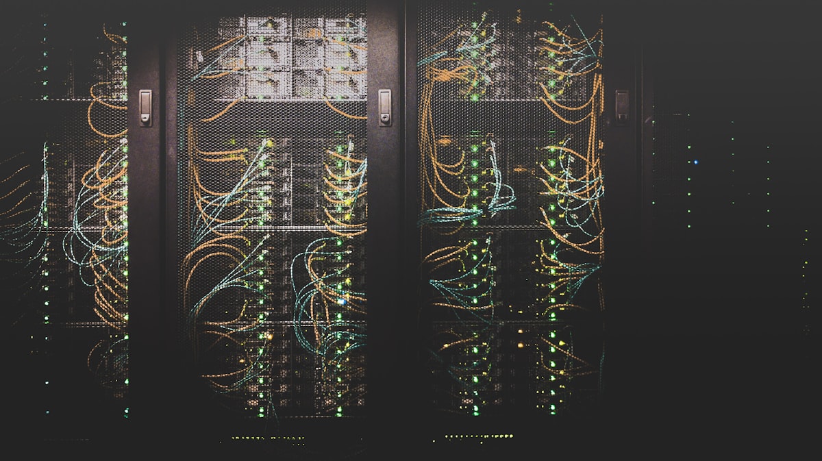
Published ahead of NVIDIA GTC 2026 (San Jose, March 16-19)
Updated March 16, 2026: NVIDIA officially rebranded ICMS to CMX (Context Memory Extensions) at GTC 2026. This post has been updated to reflect the new name. The architecture, the BlueField-4 foundation, and the G3.5 tier positioning are unchanged. CMX also introduces DOCA Memos, the SDK for managing KV cache across compute nodes with hardware-accelerated encryption, and confirms Spectrum-X Ethernet as the RDMA fabric.
The Four Eras of Keeping Bytes
Every decade, the storage industry reinvents itself. But each reinvention has shared the same core assumption: storage is about bytes. Store them, retrieve them, don’t lose them. The interface changes (SCSI, iSCSI, NFS, S3) but the contract doesn’t: you give me bytes, I give them back when you ask.
That contract is ending.
Era 1: The File (NAS, 1980s-2000s)
Network Attached Storage gave us the file abstraction. Hierarchical namespaces, POSIX semantics, NFS and SMB. It was the language of workstations, home directories, and shared drives. Files had names, permissions, and modification times. Storage understood nothing about what was inside them.
Era 2: The Block (SAN, 1990s-2010s)
Storage Area Networks stripped away even the file abstraction. Raw blocks, addressed by LUN and offset, served databases and virtual machines that needed deterministic latency and their own filesystem semantics. Storage became dumber on purpose. Block devices are maximally generic, maximally fast, and maximally ignorant of their contents.
Era 3: The Object (S3, 2006-present)
Amazon S3 reinvented storage as an HTTP API. Objects with keys, metadata, and flat namespaces. No hierarchy, no POSIX, no open/close semantics. Just PUT and GET over the internet. S3’s genius wasn’t technical. It was economic. Pay-per-request pricing, infinite namespace, and eleven nines of durability turned storage from a capital expenditure into a utility.
For nearly two decades, the entire industry orbited S3’s API. MinIO, Ceph RGW, Wasabi, Backblaze B2, Cloudflare R2. Every alternative object store exists because S3 defined the interface. The competition was on cost, performance, and deployment model. Never on capability.
Era 4: The Data (2024-)
We’re now entering the fourth era, and it breaks the pattern. For the first time, the storage system is expected to understand what it stores. Not just bytes, but rows, columns, embeddings, schemas, versions, and inference context. The contract is no longer “store my bytes.” It’s “understand my data.”
Three simultaneous shifts are driving this.
Shift 1: Tables Are Eating Object Storage
Apache Iceberg has quietly become the most consequential data infrastructure project since S3 itself.
The numbers tell the story: Iceberg adoption is projected to surpass Delta Lake within three years, with 31% current adoption and 29% planned adoption versus Delta’s 39%/23% split. The Iceberg catalog service market hit $578 million in 2024 and is projected to reach $4.18 billion by 2033, growing at 21.7% annually. Enterprises report 90% reductions in S3 API costs after migrating from Hive to Iceberg, and 20% savings on compute from more efficient query execution.
What’s happening is structural: organizations are replacing their data warehouses with Iceberg tables sitting on object storage. The lakehouse architecture (coined by Databricks, now an industry-wide movement) puts an open table format (Iceberg, Delta, Hudi) on top of S3-compatible storage and queries it directly with Spark, Trino, DuckDB, Flink, or any engine that understands the format.
This changes what object storage needs to be. An Iceberg table isn’t a single object. It’s a graph of metadata files (manifest lists, manifests, snapshots) pointing to data files (Parquet, ORC, Avro), all stored as objects. The catalog that tracks tables, schemas, and snapshots becomes the critical control plane. If your object store doesn’t speak Iceberg natively, you need an external catalog service. Another system to deploy, monitor, secure, and scale.
The hyperscalers got the memo. AWS launched S3 Tables in December 2024, the first S3 feature that understands tabular structure, with built-in Iceberg support delivering 3x faster query throughput and 10x higher TPS than self-managed tables, plus automatic compaction and snapshot management. S3 Tables added Iceberg REST Catalog APIs in March 2025, letting any Iceberg-compatible engine discover and query tables stored in S3 without an external metastore.
On the software-defined side, MinIO is the only company that has fully internalized this shift. AIStor Tables, announced GA in February 2026, embeds the full Apache Iceberg V3 Catalog REST API directly into the object store. No external Hive Metastore. No AWS Glue dependency. No separate catalog service. Tables and objects coexist in a single system. The catalog is the storage.
This is the right architectural instinct. When every analytics query begins with a catalog lookup that resolves to a set of objects, separating the catalog from the store is an artificial boundary that adds latency, complexity, and failure modes.
Shift 2: Vectors Are Becoming a Storage Primitive
The rise of RAG (Retrieval-Augmented Generation), semantic search, and AI agents has created a new data type that doesn’t fit any existing storage abstraction: the vector embedding.
An embedding is a fixed-length array of floating-point numbers (typically 256-2048 dimensions) that represents the semantic meaning of a piece of content. A document paragraph, an image, a code snippet, a customer interaction. Querying vectors means finding the nearest neighbors in high-dimensional space, not matching keys or scanning columns.
The first generation of vector databases (Pinecone, Weaviate, Qdrant, Milvus) built purpose-built systems for this workload. But as embedding counts scale into the billions, a pattern is emerging: vector storage is converging back into object storage.
AWS made this explicit with S3 Vectors, launched in preview in 2025 and generally available in December 2025 with support for 2 billion vectors per index. S3 Vectors reduces vector storage and query costs by up to 90% compared to purpose-built vector databases, delivers sub-second query latency for infrequent access patterns, and integrates natively with Amazon Bedrock for RAG workflows.
The takeaway is clear: vectors aren’t a separate workload that needs a separate database. They’re a data type that belongs in the same store as the objects and tables they index. A document lives in object storage. Its Iceberg-managed metadata lives in a table. Its embedding lives in a vector index. All three should be in the same system, governed by the same policies, replicated by the same engine, and queried through the same endpoint.
No software-defined object store handles this today. The ones that recognize the convergence first will define the next decade.
Shift 3: NVIDIA Is Building a New Memory Tier
At CES 2026, Jensen Huang announced something that most storage coverage buried under GPU hype: a new tier in the memory hierarchy, originally called ICMS and now officially branded CMX (Context Memory Extensions). CMX is not a storage product. It rewrites the relationship between GPUs and storage.
The Memory Hierarchy for AI Inference
NVIDIA’s Rubin platform defines five tiers for inference data:
| Tier | Medium | Access Time | Purpose |
|---|---|---|---|
| G1 | GPU HBM | Nanoseconds | Active token generation |
| G2 | Host System RAM | Microseconds | KV cache staging, prefill buffers |
| G3 | Local NVMe SSDs | ~100 microseconds | Warm KV cache, short-term reuse |
| G3.5 (CMX) | Ethernet-attached flash | Low microseconds (RDMA) | Shared KV cache across pods |
| G4 | Shared Object Storage | Milliseconds | Durable artifacts, checkpoints, datasets |
The breakthrough is G3.5. Traditional inference offloads KV cache from GPU HBM to host RAM (G2) or local SSD (G3). But these are per-node resources. When Agent A builds a 128K-token context on Node 1, and Agent B needs a related context on Node 7, there’s no shared tier. The context must be recomputed from scratch.
CMX solves this with a pod-level shared flash tier, powered by BlueField-4 DPUs with 800 Gb/s connectivity, RDMA-accelerated NVMe-oF transport via Spectrum-X Ethernet, and purpose-built KV cache management via NVIDIA Dynamo, NIXL (NVIDIA Inference Transfer Library), and DOCA Memos for hardware-accelerated KV cache APIs.
The performance claims are striking: 5x higher tokens-per-second and 5x better power efficiency compared to traditional storage approaches for long-context inference. The key insight is that KV cache is transient, derived, and recomputable. It doesn’t need the durability guarantees of traditional storage, but it needs the bandwidth and shareability that local SSDs can’t provide.
What This Means for Storage Systems
CMX doesn’t replace object storage. It creates a new tier above it in the latency hierarchy and below it in the durability hierarchy. The infrastructure looks like:
┌──────────────────────────────────────────────────┐
│              GPU Cluster (Rubin Pods)             │
│  G1: HBM  ←→  G2: Host RAM  ←→  G3: Local NVMe  │
│                      ↕                            │
│         G3.5: CMX (BlueField-4 + Flash JBOFs)     │
│         Shared KV cache, RDMA, NVMe-oF            │
│                      ↕                            │
│        G4: Object Storage (S3-compatible)          │
│        Training data, checkpoints, Iceberg tables  │
│        Vector indexes, model artifacts             │
└──────────────────────────────────────────────────┘
G4, the object storage layer, is still the foundation. It holds the durable data: training datasets, model weights, fine-tuning artifacts, Iceberg-managed analytics tables, vector embeddings, and RAG corpora. CMX doesn’t replace any of this. What it does is create a new consumer of object storage, one that pre-stages context from G4 into G3.5 for rapid inference access.
The downstream effects are significant:
-
Object storage must be fast enough to feed CMX. If the G4 tier can’t deliver data to G3.5 at wire speed, the entire memory hierarchy stalls. Slow object storage becomes the bottleneck for inference latency.
-
Object storage must understand data semantics. CMX doesn’t want raw bytes. It wants KV cache blocks, embedding chunks, and context windows. The storage system that can organize, index, and pre-stage this data based on inference patterns will outperform one that treats everything as opaque objects.
-
The storage vendor ecosystem is mobilizing. NVIDIA named storage partners for CMX at launch: DDN, Dell, HPE, Hitachi Vantara, IBM, NetApp, Nutanix, Pure Storage, Supermicro, VAST Data, and WEKA among them. Conspicuously, no software-defined object storage project is on that list. The CMX ecosystem is being built by proprietary vendors.
At GTC 2026 (today), NVIDIA confirmed the CMX rebrand and deepened the Dynamo + CMX integration story. The storage systems that integrate with this stack (speaking NVMe-oF, understanding KV cache semantics, delivering RDMA-capable throughput via Spectrum-X) will be positioned as the G4 foundation for the next generation of AI infrastructure.
The Convergence: What the Next Storage System Must Be
These three shifts (tables, vectors, and inference context) are not separate trends. They’re converging into a single requirement: the storage system must understand data, not just bytes.
What that looks like in practice:
1. Native Table Support (Iceberg)
The storage system must embed an Iceberg REST Catalog, manage table metadata (snapshots, manifests, schema evolution), and perform automatic maintenance (compaction, orphan file cleanup, snapshot expiration). Tables are not a separate product. They’re a view of the same objects.
AWS understood this with S3 Tables. MinIO understood this with AIStor Tables. The next software-defined storage system must understand it too.
2. Native Vector Support
Vector embeddings must be a first-class storage primitive, not a separate database that happens to use the object store as a backend. Store vectors, query nearest neighbors, and link embeddings to their source objects and table rows, all through the same API.
AWS understood this with S3 Vectors. No one else has followed.
3. CMX-Ready Performance
The G4 tier must deliver sustained, high-bandwidth reads to feed CMX pre-staging. This means:
- RDMA-capable networking (RoCEv2, with Spectrum-X compatibility)
- NVMe-oF support for direct flash access
- Erasure-coded reads that can saturate 100+ Gb/s links
- Latency-optimized metadata lookups for context-aware pre-staging
4. Schema-Aware Replication and Governance
When storage understands tables and vectors, replication becomes semantic: replicate a table’s latest snapshot (not individual Parquet files), replicate an embedding index (not individual vector blobs), apply retention policies to table versions (not object prefixes). Governance becomes meaningful: column-level access control in Iceberg tables, embedding visibility policies for multi-tenant RAG, audit trails that reference table operations rather than raw PUTs and GETs.
5. Single System, Single Endpoint
The worst outcome is the current state: one system for objects, another for tables, another for vectors, and a proprietary appliance for KV cache. Each with its own API, its own consistency model, its own failure modes, its own monitoring stack.
The right outcome is a single system that stores objects, manages Iceberg tables over those objects, indexes vectors alongside them, and serves as the durable foundation for CMX-accelerated inference. All through one endpoint, on one cluster, with one operational model.
Who Gets It?
Let’s be honest about the competitive landscape.
The hyperscalers get it. AWS is systematically expanding S3 from “object store” to “data platform.” S3 Tables for Iceberg, S3 Vectors for embeddings, S3 Express One Zone for low-latency inference data. Each launch makes S3 harder to leave. That’s the point.
MinIO gets it. They’re the only software-defined storage company with no hardware lock-in that has shipped native Iceberg V3 support (AIStor Tables, GA February 2026), articulated a coherent lakehouse-on-object-storage strategy, and positioned their product as a data platform rather than just a byte store. AB Periasamy and the MinIO team have consistently been 12-18 months ahead of the rest of the software-defined storage world in recognizing architectural shifts.
The traditional storage vendors are adapting. Dell, Pure, NetApp, and VAST Data are all part of NVIDIA’s CMX partner ecosystem. But their advantage is integration agreements, not architecture. They’re adding Iceberg support, adding vector capabilities, and adding RDMA endpoints to existing products. Bolted on, not built in.
The rest of the software-defined world doesn’t get it. Ceph is still arguing about RGW performance. SeaweedFS is focused on POSIX compatibility. Garage is optimizing for self-hosting. These are all valid goals, but they’re goals from Era 3. The data-aware storage system (the one that speaks Iceberg, indexes vectors, and feeds NVIDIA’s inference pipeline) doesn’t exist yet in the software-defined world outside of MinIO’s commercial offering.
The Opportunity
There is a gap in the market that is about to become a chasm.
On one side: AWS, building the definitive data platform but locking it inside their cloud. On the other: MinIO, building the on-premises alternative but as a commercial product with enterprise licensing.
In between: no software-defined, cloud-native, data-aware object storage with no hardware lock-in that natively handles Iceberg tables, vector indexes, and CMX-ready inference workloads. No system that an organization can deploy on their own hardware, on any cloud, and use as the foundation for both analytics and AI.
The infrastructure stack that Jensen Huang will showcase at GTC 2026 (Rubin GPUs, BlueField-4 DPUs, Dynamo inference framework, Spectrum-X networking, and CMX) needs a G4 layer. NVIDIA doesn’t build storage. They build partnerships with storage vendors. The question is whether that G4 layer will be a proprietary appliance from a traditional vendor, a hyperscaler lock-in play, or a software-defined data platform with no hardware lock-in that runs anywhere.
Storage is no longer about storage. It’s about data. The system that understands this, that treats tables, vectors, and inference context as native citizens rather than afterthoughts, will define the next era.
The first three eras were about how to store bytes efficiently. The fourth era is about what those bytes mean.
NVIDIA GTC 2026 runs March 16-19 in San Jose. Jensen Huang’s keynote is Monday, March 16, 8-11 AM PDT. CMX (formerly ICMS) details from the NVIDIA CMX page, NVIDIA Technical Blog, and NVIDIA Newsroom. MinIO AIStor Tables coverage from Blocks and Files and MinIO Blog. Apache Iceberg adoption data from the 2025 State of the Iceberg Ecosystem survey. Amazon S3 Tables announcement and S3 Vectors GA announcement. NVIDIA Dynamo documentation.