A Field Guide to Storage Protocols in the AI Era

Network infrastructure and data connections

Every storage protocol you need to understand, why it exists, and which ones will survive the next decade.

Start Here: What Is a “Storage Protocol” Anyway?

Before we get into it, let’s agree on terms. A storage protocol is the language a computer uses to talk to the thing holding its data. It defines how bytes get from Point A (your application) to Point B (a disk, a flash chip, a cloud bucket, a GPU’s memory). Different protocols exist because Point B keeps changing, and so does what we’re asking it to do.

Think of it like ordering food. You can walk into the kitchen and grab it yourself (local storage). You can call a waiter (a network protocol). You can use a delivery app (cloud API). Each method has trade-offs in speed, convenience, and how much control you have over what arrives.

The AI revolution didn’t invent new physics. Data still lives on magnetic platters, flash cells, or DRAM chips. But it did change what “fast enough” means, how much data we’re moving, and where it needs to go. Let’s walk through every layer.

Layer 1: Local Storage, the Drives Themselves

Hard drives and storage hardware

Local storage means a physical device plugged directly into your machine. No network, no middleman. Three technologies dominate.

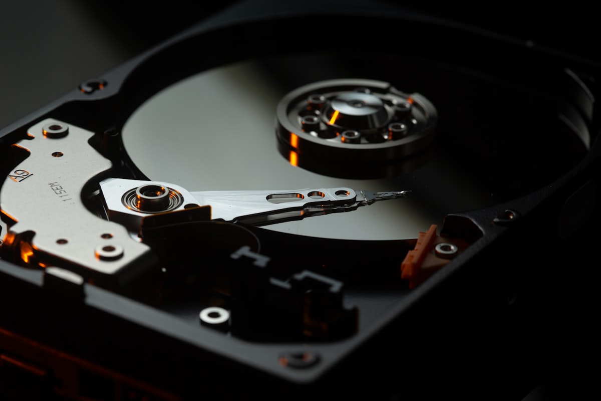
Hard Disk Drives (HDDs)

A spinning metal platter coated in magnetic material, with a tiny arm that floats nanometers above the surface reading and writing data. The same basic design since IBM shipped the first one in 1956 (it was the size of two refrigerators and held 5 MB).

How they work. The arm seeks to a position on the platter, waits for the right sector to spin underneath, and reads or writes magnetically. This mechanical motion is why HDDs have seek times measured in milliseconds. The arm literally has to move.

Speed. Sequential reads around 200-250 MB/s for modern drives. Random I/O is the killer: maybe 100-200 IOPS because each operation requires a physical seek.

Where they still win. Cost per terabyte. An 18TB HDD costs around $250. That’s roughly $0.014/GB. Nothing else comes close for bulk capacity. Cold archives, backup targets, surveillance footage, regulatory retention. Any workload where you need petabytes and can tolerate latency.

AI relevance. HDDs still hold the majority of the world’s training data in cold storage tiers. The dataset you download from Hugging Face probably lived on spinning rust before it reached you.

Solid State Drives (SSDs, SATA)

No moving parts. Data is stored in NAND flash cells: tiny transistors that trap electrons to represent bits. SATA SSDs plug into the same connectors that HDDs use, which made them a drop-in upgrade starting around 2010.

How they work. Flash cells are organized into pages (4-16KB) and blocks (256-512 pages). You can read or write individual pages, but you can only erase an entire block at once. This asymmetry (read a page, erase a block) is the source of most SSD complexity. A chip called the Flash Translation Layer (FTL) manages the mapping.

Speed. SATA tops out at 600 MB/s (the interface is the bottleneck, not the flash). Random IOPS around 50,000-100,000.

AI relevance. Minimal for training workloads. SATA’s 600 MB/s ceiling is a hard wall. But plenty of inference servers still have SATA SSDs for the OS and model weight storage where latency isn’t the primary concern.

NVMe SSDs: The Game Changer

NVMe (Non-Volatile Memory Express) is what happens when you throw away the legacy interface and design a protocol specifically for flash. Instead of talking through the SATA/AHCI stack (designed for spinning disks), NVMe talks directly over PCIe lanes, the same high-speed bus your GPU uses.

How they work. Same NAND flash as SATA SSDs, but the protocol supports 65,535 queues with 65,536 commands each (vs SATA’s single queue of 32 commands). That’s the difference between a single-lane road and a 65,535-lane highway.

Speed. PCIe Gen4 x4: 7 GB/s reads. Gen5 x4: 14 GB/s. Random IOPS: 1,000,000+. A single NVMe drive is faster than an entire rack of HDDs.

Form factors. M.2 (the little stick in your laptop), U.2 (2.5” enterprise), and the newer EDSFF (ruler-shaped, designed for maximum density: 32 drives in 1U for 4+ PB in less than 2 inches of rack space).

AI relevance. This is where it gets interesting. A single GPU training run might read hundreds of terabytes. NVMe’s bandwidth means a node with 24 drives can deliver 168 GB/s to local applications. That’s enough to feed multiple GPUs without starving them. NVIDIA’s GPUDirect Storage (GDS) can even bypass the CPU entirely. Data flows straight from NVMe to GPU memory over PCIe.

The cost. NVMe is 3-5x the price per TB of HDDs. But price-per-IOPS and price-per-GB/s tell a completely different story. For performance-sensitive workloads, NVMe is the cheapest option by far.

Layer 2: Making Remote Storage Feel Local

Here’s where it gets fun. What if the storage isn’t physically in your server but you want your applications to think it is?

Direct-Attached Storage (DAS)

DAS is technically “remote” in the sense that the drives live in a separate enclosure (a JBOD, Just a Bunch of Disks), connected to your server by a cable. But the connection is direct, not over a network. Common interfaces include SAS (Serial Attached SCSI) cables that can connect 100+ drives to a single server.

Think of it as an extension cord for your storage. Your server sees the drives as if they were internal. No network stack, no shared access. Simple, fast, cheap.

AI use case. DAS JBOFs (Just a Bunch of Flash) are the storage backbone of many GPU training clusters. NVIDIA DGX systems ship with NVMe SSDs as DAS. When you need raw bandwidth without network overhead, DAS wins.

Network-Attached Storage (NAS) and NFS

NAS puts storage on the network and exposes it as a file system. Your server mounts a remote share and accesses files with standard read/write/open/close operations, the same POSIX semantics as a local filesystem.

The protocol. NFS (Network File System), invented by Sun Microsystems in 1984, is the Unix standard. SMB/CIFS is the Windows equivalent. NFSv4.1+ adds parallel NFS (pNFS) for distributing data across multiple servers.

How it feels. You mount -t nfs server:/export /mnt/data and then ls /mnt/data like it’s local. Applications don’t know the difference. That’s the magic, and the trap.

The trap. POSIX file semantics (locks, permissions, open-close-delete atomicity) are expensive to maintain over a network. Every stat() call, every directory listing, every lock check crosses the network. At scale, metadata operations become the bottleneck, not data transfer.

AI relevance. NFS is the most common protocol for AI training data today. Why? Because PyTorch’s DataLoader, TensorFlow’s tf.data, and every ML framework expect a filesystem path. dataset = ImageFolder("/mnt/training-data/") just works. No special SDK, no API calls, no code changes. This simplicity is NFS’s superpower.

Here’s the dirty secret: NFS is often not the right protocol for AI workloads. Training data is read sequentially, shuffled, and never modified. POSIX semantics (locks, permissions, mtime tracking) are pure overhead. But NFS persists because changing the data loading code is friction, and engineers optimize for “works today” over “optimal tomorrow.”

Layer 3: Block Storage, the SAN Era

What Is Block Storage?

Block storage strips away the file abstraction entirely. No filenames, no directories, no permissions. Just numbered blocks (typically 512 bytes or 4KB) on a logical volume. The server sees a raw disk and puts its own filesystem on top.

Think of it as renting an empty apartment. The building (SAN) provides the space, but you bring your own furniture (filesystem) and organize it however you want.

The Rise of the SAN

Storage Area Networks emerged in the late 1990s when databases outgrew local storage. The idea: build a dedicated high-speed network just for storage traffic, separate from the regular Ethernet LAN.

The protocols:

Fibre Channel (FC). The original SAN protocol. Dedicated switches, dedicated cables (fiber optic), dedicated HBAs (Host Bus Adapters). Blazing fast for its era (1 Gb/s in 1997, 64 Gb/s today). Extremely reliable. Extremely expensive. Think of FC like a private highway: fast and uncongested, but you have to build the entire road yourself.
iSCSI. “Let’s run SCSI commands over regular Ethernet.” Launched in 2003, iSCSI democratized SANs. Instead of dedicated FC infrastructure, you use your existing network. Slower than FC (Ethernet has more overhead), but dramatically cheaper. The Honda Civic to FC’s Ferrari.
Fibre Channel over Ethernet (FCoE). An attempt to get FC’s performance on Ethernet’s infrastructure. Required special “lossless” Ethernet switches. Never gained traction. It combined the complexity of both protocols with the advantages of neither.

A Brief History of SAN Drama

The SAN era (roughly 2000-2015) was the golden age of enterprise storage vendors. EMC (now Dell EMC), NetApp, IBM, Hitachi, Pure Storage. These companies built empires selling SAN arrays that cost more than sports cars. A fully loaded EMC Symmetrix could run $5 million. The sales cycle involved steak dinners and golf outings. Storage admins had dedicated SAN teams.

What made SANs dominant was databases. Oracle, SQL Server, DB2: all needed consistent, low-latency block I/O. A SAN could deliver sub-millisecond latency with enterprise features like snapshots, replication, thin provisioning, and deduplication. Try doing that with a pile of local disks.

The decline. The cloud changed everything. AWS EBS (Elastic Block Store) is essentially a cloud SAN (block volumes over the network) but you don’t buy the hardware, configure the switches, or hire the SAN admin. On-premises SANs still exist (banks, hospitals, government), but new deployments are increasingly cloud-based or replaced by software-defined alternatives.

AI relevance. Block storage is critical for databases that support AI workflows: PostgreSQL for metadata, vector databases like pgvector, ML experiment tracking. But you don’t train models on block storage. The block interface (read block 47,382 from LUN 3) is a terrible match for “stream 50TB of images sequentially.”

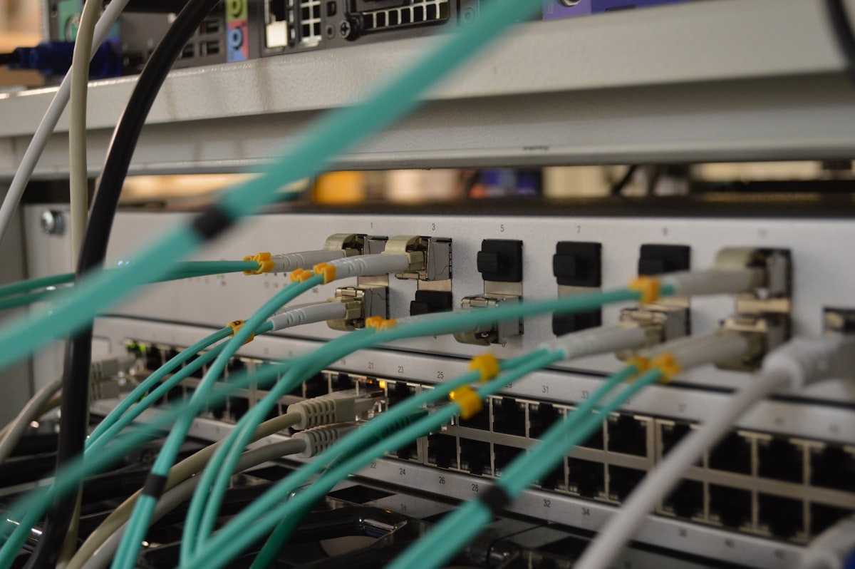
Layer 4: NVMe over Fabrics, the SAN Reborn

NVMe-oF is the modern answer to the SAN. The concept: extend the NVMe protocol over a network, so remote flash drives appear as if they’re locally attached. Microsecond-level remote storage access.

Why NVMe-oF Exists

Local NVMe is fast: 10 microsecond latency. But what if you have 1,000 NVMe drives in a rack and 100 compute nodes that need access? You can’t plug every drive into every server. NVMe-oF extends the NVMe queuing model over a network fabric, preserving the multi-queue architecture that makes NVMe fast.

The Transport Options

Transport	Latency Added	Infrastructure Required	Reality Check
RDMA (RoCEv2)	~5-10 us	Lossless Ethernet (PFC/ECN), specialized NICs	Fastest, but configuring lossless Ethernet correctly is an art form. Misconfigure one switch and performance craters.
InfiniBand	~2-5 us	Dedicated InfiniBand switches and HCAs	HPC standard, NVIDIA’s home turf. Fast and reliable, but separate network fabric.
TCP	~30-80 us	Standard Ethernet	Easy to deploy, works everywhere. But 30-80us on top of NVMe’s 10us is a 3-8x latency hit. Still way faster than iSCSI.

The Promise vs. Reality

The promise. “Remote NVMe that feels local.” Disaggregated storage: separate your compute and storage into independent pools that scale independently.

The reality in 2026. NVMe/TCP works and is widely deployed, but “feels local” is a stretch when you 3x the latency. RDMA is genuinely close to local performance, but requires careful network engineering. InfiniBand delivers on the promise, but only within HPC/AI clusters that already run InfiniBand for GPU-to-GPU communication.

AI relevance. This is big. NVIDIA’s entire inference infrastructure assumes NVMe-oF as the transport between storage and compute. BlueField-4 DPUs speak NVMe-oF natively. When Jensen Huang talks about “AI factories,” the storage fabric connecting thousands of GPUs to petabytes of flash is NVMe-oF over InfiniBand or RoCEv2.

Layer 5: Object Storage, the Quiet Revolution

Fiber optic cables representing modern data transport

What Object Storage Is

Object storage throws away everything you know about filesystems and block devices. No hierarchy. No directories. No block addresses. Just three things:

A key (a string, like training-data/imagenet/n01440764/n01440764_10026.JPEG)
The data (the bytes)
Metadata (arbitrary key-value pairs describing the object)

You interact with it through HTTP: PUT to store, GET to retrieve, DELETE to remove, LIST to enumerate. That’s essentially the whole API.

The Origin Story

Amazon launched S3 (Simple Storage Service) on March 14, 2006. It was designed for one thing: giving web applications a place to store files without managing servers. Upload a profile photo, serve a static website, store log files. Nobody was thinking about AI.

Why S3 won. Three things that sound boring but changed everything:

Pay per use. No upfront hardware purchase. Store one byte or one petabyte, pay only for what you use.
Infinite namespace. No capacity planning. No “disk full” errors. Just keep writing.
Eleven nines of durability. 99.999999999%. Meaning if you store 10 million objects, you’d statistically lose one every 10,000 years.

The “Slow” Reputation

For its first decade, object storage had a reputation problem: it was slow. And honestly? It was. Early S3 latency was 50-200ms per request. You couldn’t run a database on it. You couldn’t mount it as a filesystem without hideous performance. It was “archive tier,” the place you put data when you didn’t need it anytime soon.

The reasons were architectural: HTTP overhead, eventually consistent reads (until 2020, S3 could return stale data after a write), and the simple fact that it was designed for throughput and durability, not latency.

The Transformation

Everything changed between 2020 and 2025:

Strong consistency (2020). S3 became strongly consistent at no extra cost. Read-after-write consistency for all operations. This single change eliminated the #1 objection from serious workloads.
S3 Express One Zone (2023). Purpose-built for latency-sensitive workloads. Single-digit millisecond first-byte latency. 10x faster than standard S3.
S3 Tables (2024). Native Apache Iceberg support. Object storage that understands tabular data. 3x faster queries, automatic compaction, built-in catalog.
S3 Vectors (2025). Native vector embedding storage and nearest-neighbor search. Sub-second queries over 2 billion vectors.
Performance at scale. Modern object stores (MinIO, Ceph RGW, and cloud-native ones) can deliver 100+ GB/s aggregate throughput on commodity hardware. That’s enough to feed a rack of GPUs.

Why Object Storage Is the Future

Here’s the contrarian take that’s rapidly becoming consensus: object storage will eat everything.

Not because it’s the fastest protocol for every workload. It isn’t. But because it solves the problems that actually matter at scale:

Scale without limits. Filesystems break at billions of files (ask anyone who’s run ls on a directory with 10 million entries). Block storage requires LUN management and capacity planning. Object storage scales to trillions of objects by design. Flat namespace, hash-based distribution, no directory tree to maintain.
Economics. Object storage on commodity hardware costs 1/10th of enterprise SAN storage. Erasure coding gives you 11-nines durability at 1.5x raw capacity (vs. 3x for replication).
HTTP is universal. Every language, every platform, every cloud speaks HTTP. No special drivers, no kernel modules, no vendor lock-in (assuming S3-compatible API).
Metadata is first-class. Unlike block and file storage, every object carries its own metadata. This is transformative for data management. Search, classify, govern, and lifecycle data based on its properties, not its location in a directory tree.
Immutability is natural. Objects are written once and read many times. This aligns perfectly with training datasets, model checkpoints, audit logs, and regulatory archives. No in-place updates means no corruption, no locking, no read-write conflicts.

Layer 6: Data Lakes and Data Lakehouses

The Data Lake

A data lake is a fancy name for “dump everything into object storage and figure out the schema later.” Coined by Pentaho CTO James Dixon around 2010, the idea was to store raw data (structured, semi-structured, unstructured) in its native format on cheap storage (originally HDFS, now mostly S3-compatible object storage).

The appeal. No upfront schema design. No ETL pipeline to transform data before loading. Just dump your CSV files, JSON logs, Parquet tables, images, and videos into buckets. Analyze later with Spark, Presto, or Hive.

The problem. Data lakes became data swamps. Without schema enforcement, governance, or quality checks, organizations ended up with petabytes of data nobody could find, trust, or use. “Schema on read” sounds liberating until you realize nobody documented the schema.

The Data Lakehouse

The lakehouse architecture (Databricks coined the term in 2020) is the fix. It puts a structured table format (Apache Iceberg, Delta Lake, or Apache Hudi) on top of object storage. You get:

Schema enforcement. Data types, column constraints, NOT NULL rules.
ACID transactions. Atomic writes across multiple files.
Time travel. Query data as it existed at any point in the past.
Partition evolution. Change how data is organized without rewriting it.
Open format. Parquet files on object storage, readable by any engine.

Why it matters for AI. A lakehouse is where training data lives in production. Your ML pipeline reads from Iceberg tables on object storage, trains a model, writes evaluation metrics back to another table, and stores model artifacts as objects. All in the same system.

The progression looks like this:

Raw data (logs, events, sensors)
        |
        v
Object Storage (S3-compatible, durable, cheap)
        |
        v
Iceberg Table (schema, versioning, ACID)
        |
        v
Feature Engineering (Spark, Flink, DuckDB)
        |
        v
Training Pipeline (PyTorch DataLoader)
        |
        v
Model Artifacts -> back to Object Storage

Everything in this pipeline speaks object storage. The lakehouse doesn’t replace S3. It adds structure on top of it. This is why object storage is the foundation layer that everything else builds on.

The NVIDIA Factor: Why This All Matters for AI

GPU cluster and AI computing infrastructure

NVIDIA doesn’t build storage. But NVIDIA increasingly dictates what storage looks like through its certification programs, reference architectures, and the sheer gravitational pull of being the center of the AI universe.

The Current State: File and Block Still Rule

Here’s something that surprises people: most AI training clusters today use NFS or Lustre for training data. Not object storage. File protocols.

Why? Three reasons:

PyTorch expects a filesystem. DataLoader(dataset=ImageFolder("/data/train/")) needs a mounted path. Rewriting data loaders to use S3 APIs is possible (via smart libraries) but adds complexity.
NVIDIA DGX and certification. NVIDIA’s validated designs (DGX SuperPOD, BasePOD) have historically certified file-based storage partners. WEKA, DDN Lustre/EXAScaler, VAST Data, NetApp: all primarily file/NFS vendors. The certification program ensures these systems can keep GPUs fed. If you want the “NVIDIA Certified” badge, you play by NVIDIA’s rules.
Random access patterns. Training with random shuffling requires random reads across a dataset. File protocols handle this naturally. Object storage traditionally adds HTTP overhead per request, making small random reads expensive.

The Shift: Object Storage Is Coming

But the tide is turning. NVIDIA’s storage ecosystem is evolving in a significant direction:

Larger datasets demand object scale. When your training set is 100TB, NFS can handle it. When it’s 10PB (common for foundation model training), you need object storage’s scale-out economics. No NFS server handles 10PB gracefully. Object storage distributes it across hundreds of nodes automatically.

Cloud training is object-native. Every major cloud’s AI training service (AWS SageMaker, Google Vertex AI, Azure ML) reads training data from object storage. Cloud-native training pipelines skip NFS entirely.

New protocols bridge the gap. S3-compatible APIs with range reads, batch operations, and prefetch hints are closing the performance gap. Libraries like AIStore, S3 connector for PyTorch, and fsspec abstract the protocol. Your DataLoader code stays the same, but reads come from S3 instead of NFS.

NVIDIA is broadening. The partner ecosystem is expanding beyond file storage. Fast object storage that can deliver sustained high-bandwidth reads to GPU clusters is becoming a validated tier. The writing is on the wall: object storage with performance guarantees will be a first-class citizen in NVIDIA’s reference architectures.

Context Memory: From ICMS to CMX

Here’s where it gets really interesting, and where most storage coverage misses the point entirely.

At CES 2026, NVIDIA announced ICMS (Inference Context Memory Storage). It’s not a product you buy. It’s a new tier in the memory hierarchy, sitting between local NVMe and shared object storage.

Why it exists. Modern AI inference (especially with large language models and AI agents) builds enormous context windows. When a chatbot maintains a 128K-token conversation, that context lives as a KV (key-value) cache in GPU memory. But GPU HBM is precious and limited. When the KV cache overflows HBM, it needs somewhere to spill.

The memory hierarchy for AI inference looks like this:

Tier	What	Latency	What Lives There
G1	GPU HBM	Nanoseconds	Active KV cache, model weights
G2	Host RAM	Microseconds	Overflow KV cache, prefill buffers
G3	Local NVMe	~100 us	Warm context, model weight shards
G3.5 (ICMS)	Network flash (RDMA)	Low microseconds	Shared KV cache across pods
G4	Object Storage	Milliseconds	Training data, checkpoints, datasets

The magic is G3.5. Without ICMS, if Agent A builds a context on Node 1 and Agent B needs related context on Node 7, it has to be recomputed from scratch. ICMS creates a shared flash tier across the pod, powered by BlueField-4 DPUs with 800 Gb/s RDMA connectivity.

The rebrand: CMX. After GTC 2026 (March 16-19, San Jose), expect NVIDIA to rebrand ICMS as CMX (Context Memory eXtensions). Same technology, better name. “ICMS” is a mouthful; “CMX” matches NVIDIA’s naming style (think CUDA, NVLink, NIM) and positions context memory as a platform extension rather than a storage product. The technology doesn’t change (BlueField-4, NVMe-oF transport, NVIDIA Dynamo orchestration) but the messaging shifts from “storage infrastructure” to “memory architecture for agentic AI.”

Why should you care? Because CMX defines what the G4 object storage layer needs to be:

Fast enough to pre-stage into CMX. If your object store can’t deliver sustained 100+ Gb/s to the CMX tier, it becomes the bottleneck for the entire inference pipeline.
Smart enough to know what to pre-stage. The object store that understands inference patterns (which context windows are reused, which model shards are hot, which datasets feed which agents) will outperform one that treats everything as opaque blobs.
Integrated with the NVIDIA ecosystem. NVMe-oF transport, GDS support, Dynamo integration. The storage system that speaks NVIDIA’s language will get the certification, the reference architecture inclusion, and ultimately the deployment.

Putting It All Together: Which Protocol for Which AI Workload?

Let’s get practical. Here’s a cheat sheet:

Data Collection and Preparation

Winner: Object Storage

Raw data arrives from everywhere: web scrapes, sensor feeds, user logs, public datasets. You need scale (petabytes), durability (don’t lose it), and cost efficiency (most of it won’t survive filtering). Object storage with lifecycle policies to tier cold data is the obvious choice.

Feature Engineering and ETL

Winner: Data Lakehouse (Object Storage + Iceberg)

Iceberg tables on object storage give you schema enforcement, versioned datasets, time travel for reproducibility, and engine-agnostic access. Run Spark or Flink for ETL, query with DuckDB for exploration, all reading from the same Iceberg tables.

Model Training

Current Winner: NFS/Lustre. Future Winner: Object Storage

Today, NFS wins because of tooling compatibility and random read performance. But as datasets grow beyond what single NFS servers can handle, and as PyTorch’s data loading ecosystem adds first-class S3 support, object storage’s scale-out architecture becomes necessary. The crossover is happening now for datasets above ~500TB.

Model Checkpointing

Winner: Object Storage

Checkpoints are large (multi-GB to TB), written periodically, and need durability. Object storage with versioning is ideal. Write checkpoint v47, keep the last 10 versions, auto-expire older ones. No filesystem to manage.

Inference: Model Serving

Winner: Local NVMe + CMX + Object Storage (tiered)

Hot model weights on local NVMe (G3). Shared context in CMX (G3.5). Model artifacts and full weight sets in object storage (G4). The tiers work together. CMX pre-stages from object storage, local NVMe caches the hottest data.

Inference: KV Cache and Context

Winner: CMX (ICMS)

This is CMX’s reason for existing. Shared, transient, high-bandwidth context that doesn’t need durability but needs to be accessible across pods. Neither NFS nor object storage is designed for this workload.

Vector Search (RAG)

Winner: Object Storage (with native vector support)

Billions of embeddings need scale-out storage, not a single-node vector database. AWS S3 Vectors showed the direction: vectors as a storage primitive, not a separate system.

The Trajectory: Where This Is All Heading

Here’s my prediction for the next five years:

NFS and block storage won’t disappear, but they’ll shrink to niche roles. NFS for legacy compatibility and small-scale training. Block for databases. Neither grows.

Object storage becomes the universal foundation. Not because it’s perfect for every workload, but because it’s good enough for most and best for scale, economics, and data management. The performance gap with file/block protocols shrinks every year. When object storage is within 20% of NFS speed but 10x cheaper at 100x the scale, the math doesn’t lie.

Table formats (Iceberg) and vector indexes become standard features of object storage, not separate products. Just as S3 absorbed consistency, it will absorb tabular and vector capabilities. MinIO’s AIStor Tables and AWS S3 Tables/Vectors are the first wave.

CMX creates a new storage category that didn’t exist before: transient, shared, high-bandwidth context memory. It’s not file, block, or object. It’s something new, purpose-built for AI inference, and it will become as fundamental to AI infrastructure as GPUs are to training.

The storage protocol that wins the AI era isn’t the fastest one. It’s the one that understands data (schemas, embeddings, inference patterns, lifecycle) rather than just moving bytes. Object storage, extended with tables and vectors and integrated with CMX, is on that trajectory. Everything else is arguing about I/O latency while the world moves to data semantics.

The bytes still matter. They always will. But the protocol that just moves bytes and nothing else? That’s the one heading for the history books.

NVIDIA GTC 2026 runs March 16-19 in San Jose. Watch for the CMX announcement during Jensen Huang’s keynote (Monday, March 16, 8-11 AM PDT). For current ICMS details, see the NVIDIA Technical Blog and BlueField-4 announcement. NVMe-oF specifications from NVM Express. Apache Iceberg at iceberg.apache.org. S3 API reference at AWS S3 documentation.